Software & Analysis
Quality 4.0: Learning quality control, the evolution of statistical quality control
Learning quality control (LQC) is a process monitoring system based on machine learning and deep learning.

Image Source: Sean Anthony Eddy/E+ via Getty Images
The Quality Show Preview: Quality 4.0 and the Zero Defects Vision
 Dr. Carlos Escobar, a research scientist at the Quality 4.0 Institute, shares his ideas combining machine learning and quality. In this talk, he introduces a new concept, learning quality control (LQC), which is the evolution of statistical quality control (SQC). This new approach allows us to solve a whole new range of engineering intractable problems.
Listen to more Quality podcasts.
Quality 4.0 is the next natural step in the evolution of quality. It is based on a new paradigm that enables smart decisions through empirical learning, empirical knowledge discovery, and real-time data generation, collection, and analysis [0]. As Quality 4.0 matures and different initiatives unfold across manufacturing companies, intractable engineering problems will be solved using the new technologies. Advancing the frontiers of manufacturing science, enabling manufacturing processes to move to the next sigma level, and achieving new levels of productivity is possible. Quality 4.0 is still in a definition phase where different authors have different perspectives on how to apply the new technologies. In this article we present learning quality control, our vision.
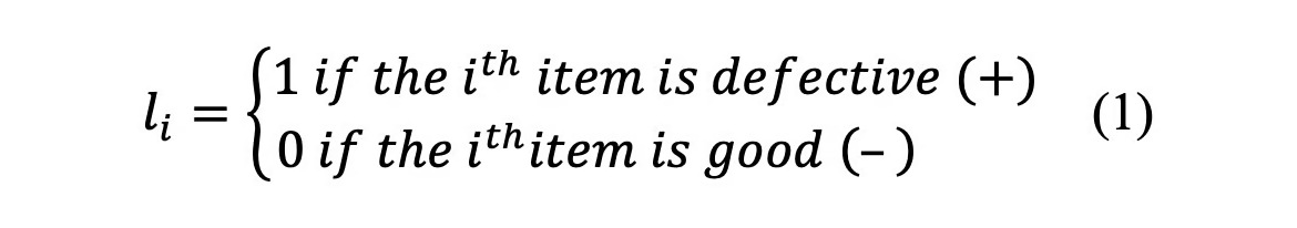
Learning quality control (LQC) is a process monitoring system based on machine learning and deep learning; for a full description, theory, implementation strategy, and examples refer to [1]. LQC focuses on real-time defect prediction or detection. The task is formulated as a binary classification problem, where historical samples (X, l) are used to train the algorithms to automatically detect patterns of concern associated to defects (e.g., anomalies, deviations, non-conformances). The historical samples include process measurements such as features (structured data), images (unstructured), or signals (unstructured) denoted by X and their associated binary quality label denoted by l ε {good defective}. Following binary classification notation, a positive label refers to a defective item, and a negative label refers to a good quality, equation 1.
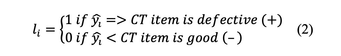
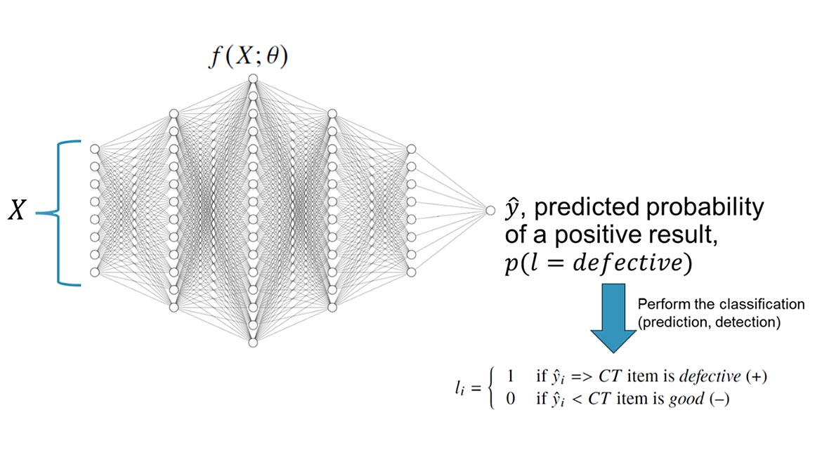
The historical samples become the learning data set used by the machine learning algorithms to train a model; learn the coefficients θ of the general form ŷ = f(X;θ) = p(l = defective), where ŷ refers to the predictive probability of the positive class (defective). Each predicted probability is compared to a classification threshold (CT) to perform the classification, equation 2.
The is defined based on the business goals considering the costs or implications of the misclassifications (errors). Figure 1 illustrates the classification process using a pretrained feed-forward neural network; depending on the problem, different machine learning algorithms are trained and tested. The performance of a classifier is summarized based on four concepts described in the confusion matrix, Table 1.
- True Negative: it refers to a good item, correctly predicted by the classifier.
- True Positive: it refers to defective item, correctly predicted by the classifier.
- False Positive: it refers to a good item incorrectly predicted to be defective. From a statistical perspective, the α error (type I) quantifies the FPs.
- False Negative: It refers to defective item incorrectly predicted to be good. The β error (type II) quantifies the FNs.
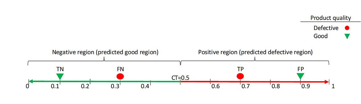
Figure 2 graphically illustrates the four concepts with respect to a . Color and geometric conventions are used to illustrate them; a red circle refers to a defective and green triangle good quality.
Binary classification of quality data sets tend to be highly imbalanced; they contain many good quality items and a few defects. Detecting or preventing those few defects is the main challenge posed by the Quality 4.0 era. Figure 3-5 graphically describe the main concepts of LQC.
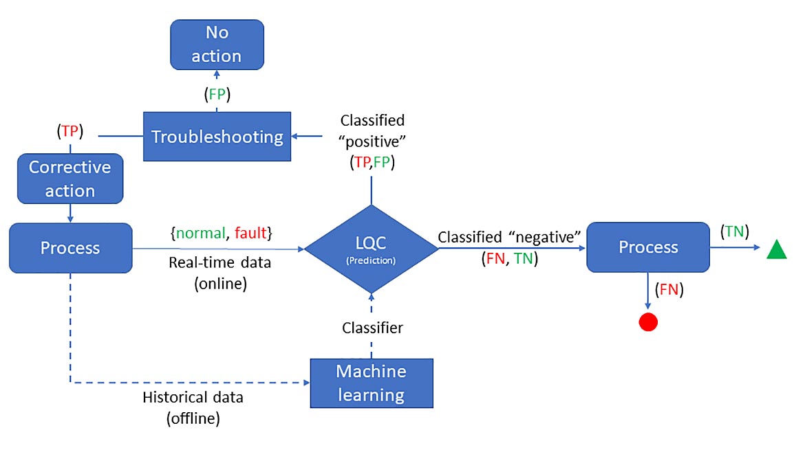
Two important concepts of LQC are explained first: (1) offline learning, historical data with the patterns of concern is used to train the machine learning algorithms to develop the classifier, this activity can last weeks or even months, (2) online deployment, the classifier is deployed into production to automatically and in real-time detect the patterns of concern associated to quality defects. Figure 3 shows an LQC monitoring system for defect prediction. Here, data from early in the process is collected to predict downstream quality issues. The positive results alert the process like a control chart, then the engineering team troubleshoots the process and generates a corrective action. Since prediction is performed under uncertainty, the FPs errors result in no corrective action but waste engineering team time and resources. The FNs or failing to detect a pattern of concern results in downstream quality issues.
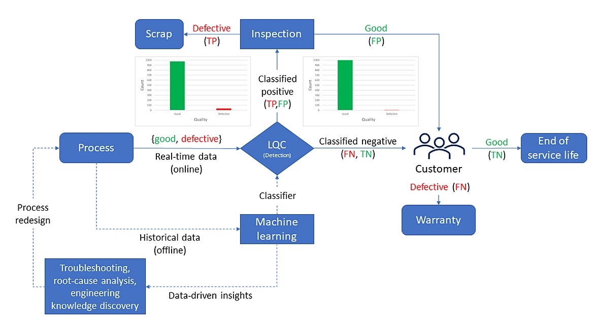
Figure 4 graphically illustrates a general manufacturing process that generates only a few defects per million opportunities. The main objective of LQC here is to detect those defective items in real-time. For example, during a welding process a signal is generated, the signal runs through a classifier to automatically detect if the weld is good or defective. All the positive results or the flagged items are sent to an inspection, the TPs are scrapped and the FP after a second inspection they may continue in the value adding process. The FNs are the main concern, as these defective items not detected would continue in the value-adding process and potentially become a warranty event or a customer complaint. In this context, whereas the FPs generate the hidden factory effect (i.e., inefficiencies), the FNs generate more serious situations. Therefore, minimizing the FNs is more important. Figure 5 shows the classification process of the LQC monitoring system in production (i.e., online deployment).
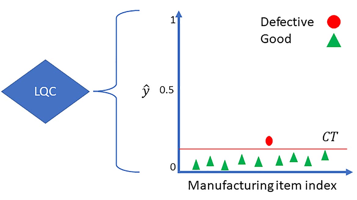
Figure 5 shows a sequence of 10 manufacturing items and their associated predicted probability of being a defect. The sixth item has a predicted probability greater than the , therefore is classified positive. Since the Binary classification of quality data sets tend to be highly imbalanced, the value is usually smaller than 0.50.
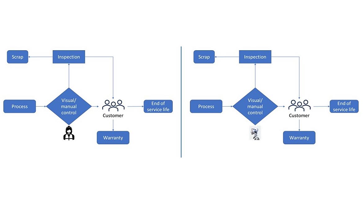
One the most promising research focus areas of Quality 4.0 is the replacement of visual or manual monitoring systems by deep learning applications. Although this leading-edge technology is already mature, surpassing human visual capabilities, in manufacturing human vision is still widely used for quality control. Deep learning allows us to reduce or eliminate monotonous and repetitive visual monitoring systems. Enabling significant improvements, especially if it is considered that due to the inherent operator biases and monotony of the task, visual or manual monitoring approaches are historically 80% accurate, Figure 6.
LQC is the evolution of statistical process control (SPC). Whereas the latter is founded on statistical methods, the former is founded on statistical methods and boosted with machine learning and deep learning algorithms, enabling the solution of a whole new range of engineering intractable problems. These algorithms have the capacity to effectively learn non-linear patterns that exist in hyper-dimensional space, surpassing traditional statistical SPC methods such as control charts. Moreover, deep learning allows us to replace human-based monitoring systems. This application was engineering intractable even a decade ago. The following section illustrates the LQC concept with a virtual case study.
Case Studies
Two virtual case studies are presented to illustrate the LQC monitoring systems. The first one is based on structured data. It demonstrates how sometimes typical control charts cannot detect patterns that exist in high dimensional spaces. In this case study, a 3D pattern is developed, thus the pattern can be seen and understood. The second case study is based on unstructured data; it illustrates how deep learning, specifically convolutional neural networks, are applied to replace visual monitoring systems.
Structured Data
A virtual case study based on structured data is presented to illustrate the LQC monitoring system, full case study presented in [2]. A pattern that exists in a 3D space that completely separates the classes is developed. The virtual data set with 10 observed values (samples) and three features is described in Table 2 and graphically visualized in Figure 7.
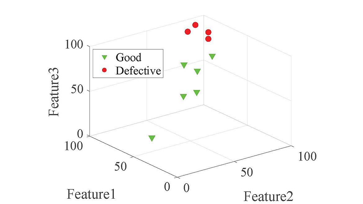
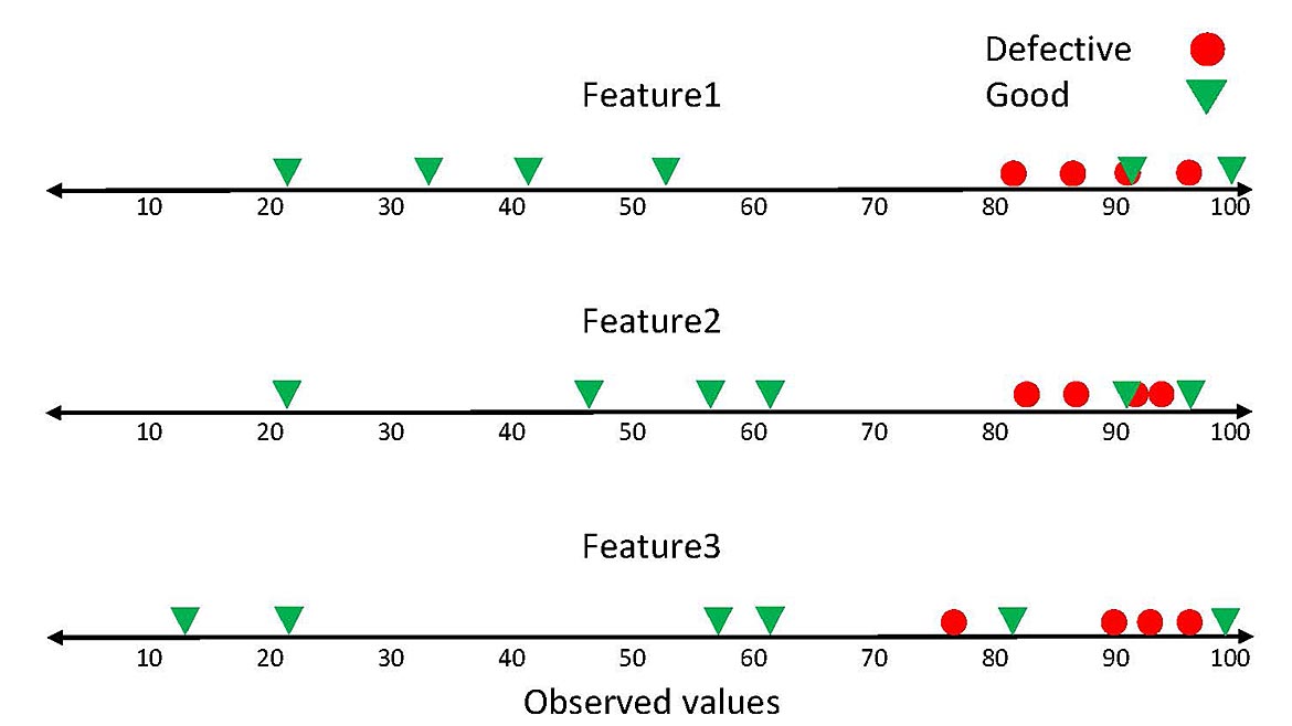
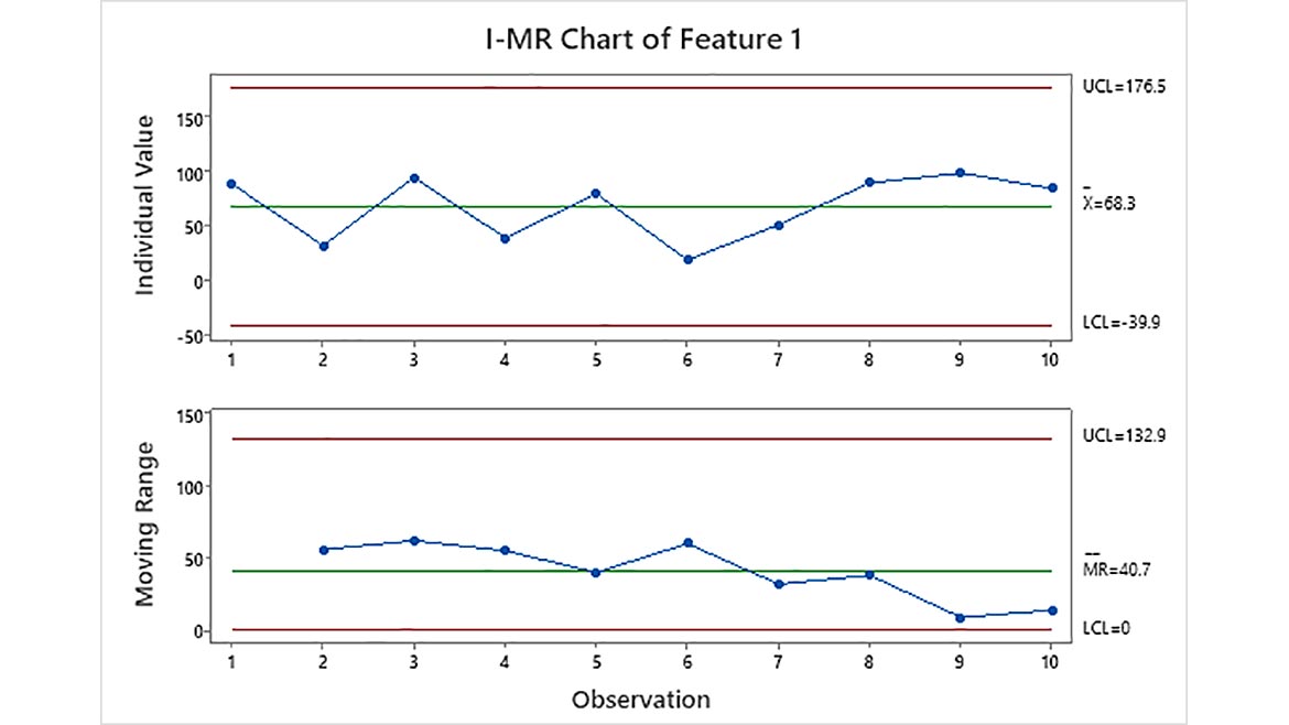
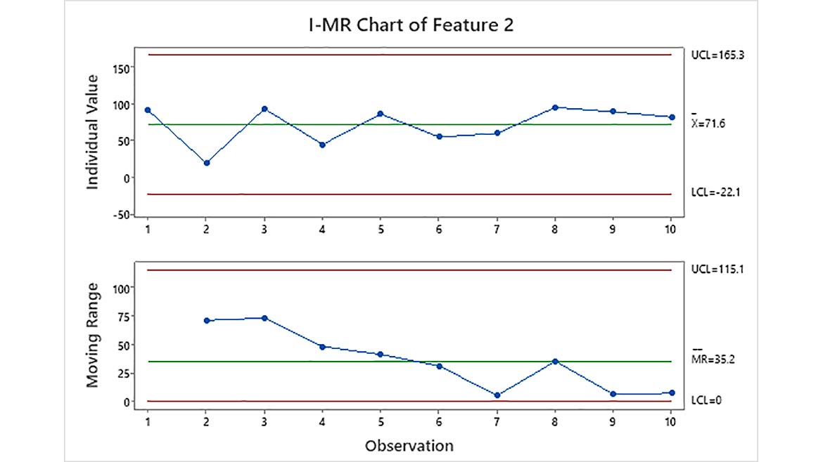
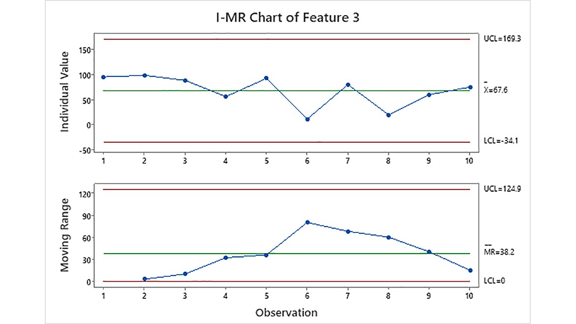
Figure 7 shows clear separation of classes in 3D, but they do not separate in 1D. As shown in the univariate analysis of Figure 8, the positive classes have high values. However, the highest value is generated by a good quality item in all the three features and the observed values between 90 and 100 of feature 1 and feature 2 have both outcomes. A univariate analysis using I-MR control chart is performed on the three features. As shown in Figure 9, no points out of control are observed.
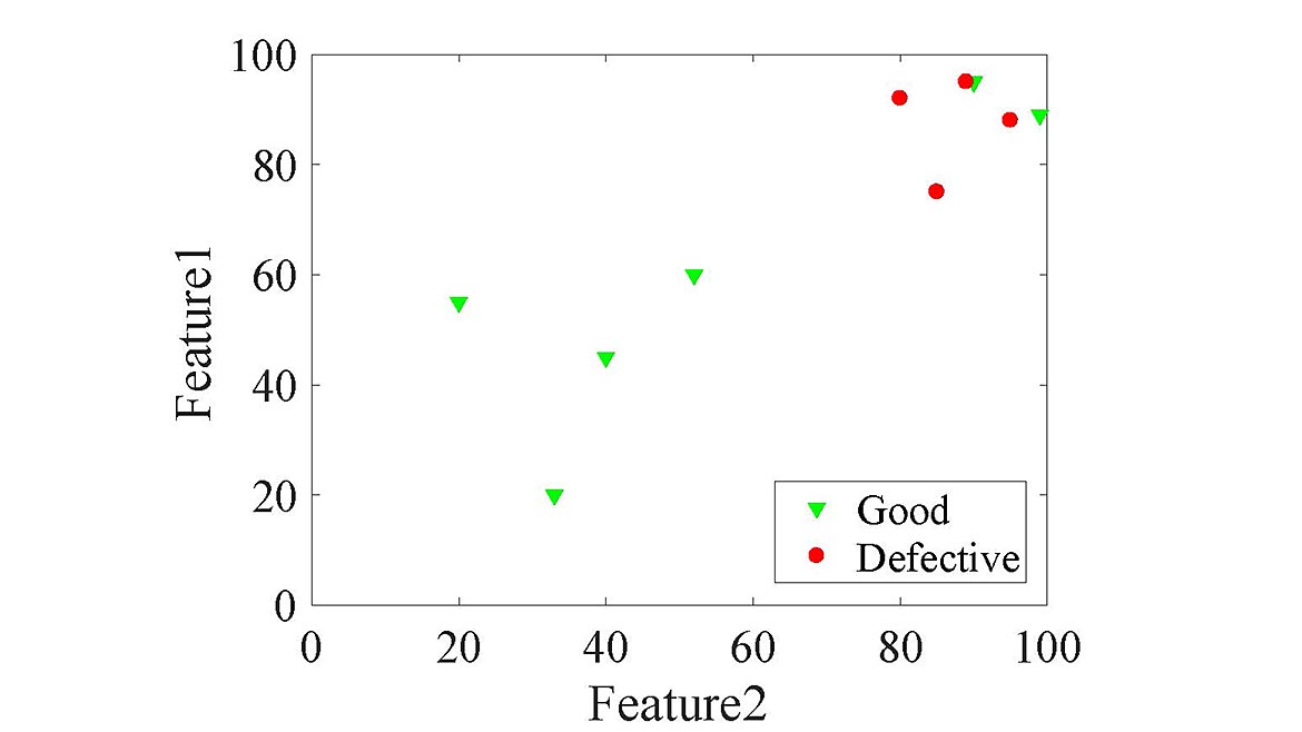
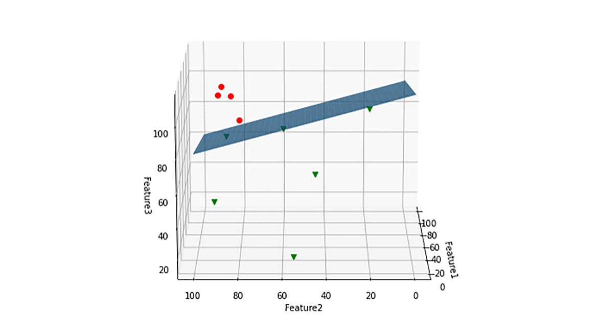
The classes do not separate in 2D. As shown in Figure 10, when the items are projected in a 2D space using feature 1 and feature 2, the defective items concentrate on the upper right; however, two good quality items exhibit the same pattern. If feature 1 is combined with feature 3, and feature 2 is combined with feature 3, the classes do not separate. But the classes show a complete separation in the 3D space. In such a case, an optimal separating hyperplane can be learned by a machine learning algorithm such as SVM. Figure 11 shows the separating hyperplane learned by the SVM using a linear kernel, for the code refer to https://github.com/Quality40/case-study-0-structured-data-. However, other algorithms such as logistic regression or neural networks can easily separate the classes in this problem.
This virtual case study is based on a simple pattern 3D pattern. However, oftentimes patterns exist in the hyper-dimensional space (e.g., 4D or higher) following non-linear relationships. In these situations, machine learning algorithms have superior capacity to learn them. For a comprehensive theory about how to train machine learning algorithms refer to the books [3,4].
Unstructured Data
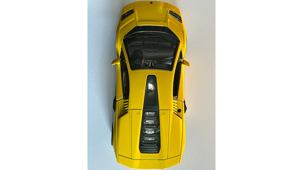
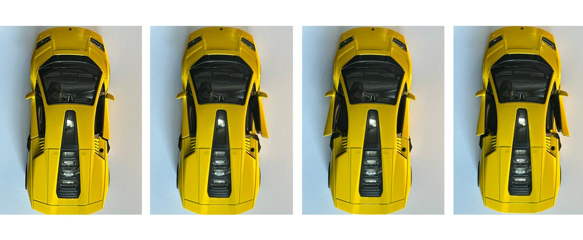
To illustrate how LQC is applied to replace visual-based monitoring systems, a virtual case study with images is presented. The task here is to train a convolutional neural networks model to automatically monitor the process to detect defects, i.e., significant deviations in the car body. Only 49 pictures were taken from a toy car replica. Figure 12 shows the good quality (i.e., negative label) and Figure 13 shows cars with significant deviations (i.e., positive labels).
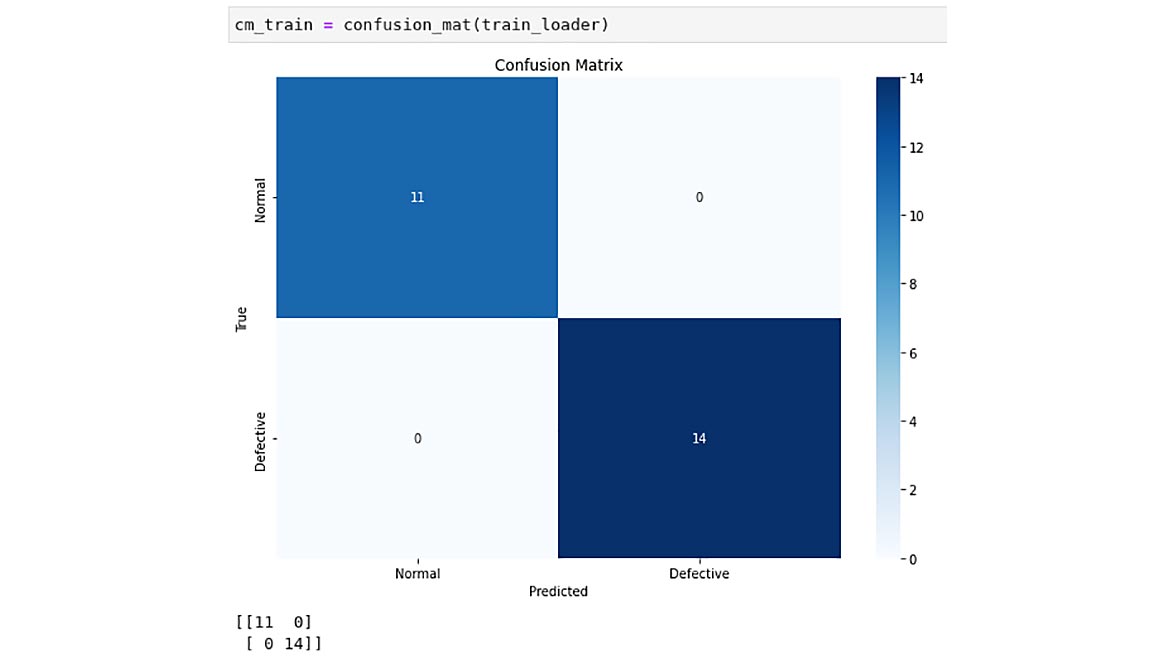
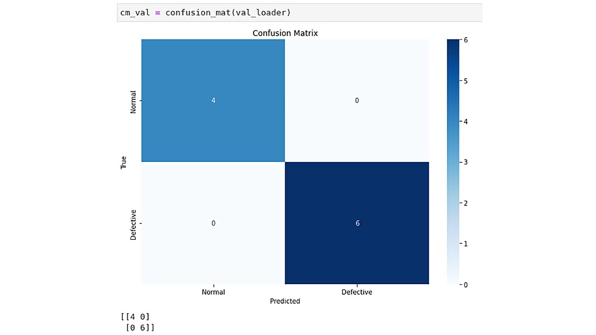
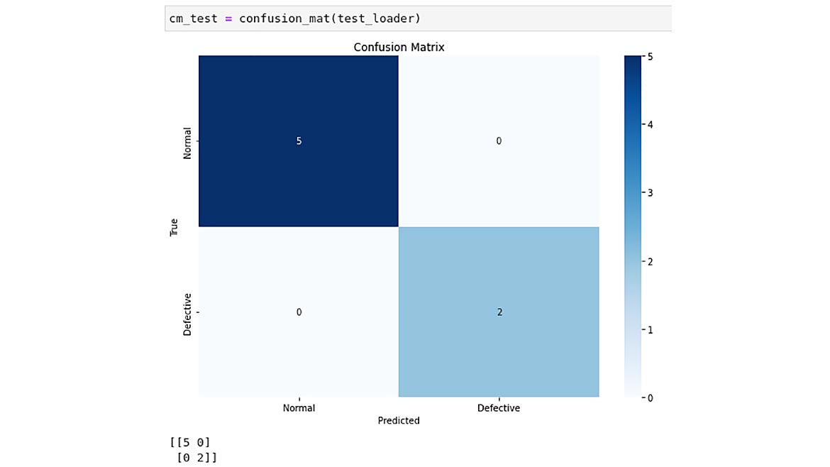
The model contains 3 convolutional layers, each with convolution kernels of size 3x3, stride 1, and padding 1, batch normalization and ReLU as activation function. The number of filters is 64, 128 and 128 for the first, second, and third convolutional layers respectively. Finally, the last convolutional activation volume is flattened and passed through a final fully connected layer with two neurons (alternatively we could only use one neuron and consider binary cross entropy as cost function). The model was trained using a constant learning rate of 0.00008 for 15 epochs, with mini batches of 2 images. The learning rate was found using random exploration, and the model was trained using the Adam optimizer. For full code implementation, refer to https://github.com/Quality40/case-study-2-unstructured-data-. Figure 14 shows the confusion matrix of the training, validation, and test sets. The model completely separates the classes.
This case study demonstrates the application of a LQC for the replacement of a visual monitoring system. The technology is ready; therefore, it is our challenge to find the applications and develop innovative solutions. The economic benefit has been widely studied, moreover, eliminating these monotonous tasks allows management to use the brainpower of the team to solve other tasks that require higher cognitive levels.
Concluding Remarks
In today’s manufacturing world, innovation is driven by Quality 4.0. However, Quality 4.0 does not replace Six Sigma. Instead, it boosts the quality movement and sets a higher knowledge bar for quality engineers. In this context, it is important to understand the nature of the problem at hand and the capabilities of each philosophy to find the most suitable approach and avoid over-complexity. The two concepts should work together cohesively, passing insights and wisdom back and forth, allowing quality professionals to drive breakthrough innovations.
Looking for a reprint of this article?
From high-res PDFs to custom plaques, order your copy today!


