Measurement
The Force of Decision Rules: Applying Specific and Global Risk to Star Wars
All Images Source: Henry Zumbrun and Morehouse Instrument Company
Decision rules are the Force of metrology. They guide us in our quest to make accurate and precise measurements, even in the face of uncertainty. But like the Force, decision rules can be complex and challenging to understand. That’s why I’m writing this article.
In this article, I will use examples from the first Star Wars movie, Episode IV: A New Hope, to demystify decision rules and make them more understandable for everyone. Specifically, I will focus on some specific and global risk examples.
Our aim is for readers grappling with the concept of measurement risk and its connection to decision rules to gain a comprehensive understanding of the fundamental principles by the conclusion of this article. Furthermore, we hope that you can put into practice some of the ideas presented here in your work within the field of metrology.
Star Wars And Measurement Uncertainty
In the expansive and mesmerizing Star Wars galaxy, where the Force ebbs and flows, epic intergalactic battles unfold, and the destinies of heroes and villains hang in the balance, the concept of measurement uncertainty and its impact on history might appear to be distant, like a star in a far-off galaxy.
However, when we take a closer look, the Star Wars saga offers profound insights into the nature of measurement uncertainty in the context of critical decisions.
These decisions range from the precision required for our fleet of X-wing fighters to hit a 2-meter target with a 0.5-meter proton torpedo when targeting the Death Star to the intricacies of using global risk models to create a clone army with remarkably low variation in overall body size.
Destroying The Death Star – Specific Risk Example
Our rebel fleet is quickly gathering after receiving the Death Star plans in which it is uncovered that a torpedo can be fired into the 2-meter exhaust port vent, which would impact the core and trigger a catastrophic explosion.
Knowing our torpedo measures 0.5 meters and the empire does not think an X-wing can get close enough to take the shot, we need to devise a plan that will ensure if we can take the shot, we will make it.
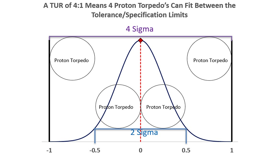
As we devise our plan, we know that the 2-meter-wide vent port would allow as many as four proton torpedoes to fit side by side.
When we discuss terms like Test Uncertainty Ratio (TUR), we are saying the measurement uncertainty is four times less than tolerance, or the tolerance is 4 times more than the measurement uncertainty.
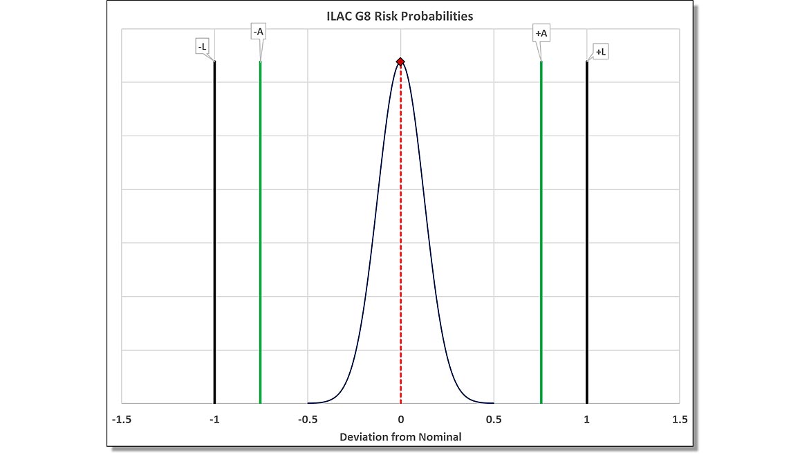
ILAC G8 defines TUR as "the ratio of the span of the tolerance of a measurement quantity subject to calibration to twice the 95% expanded uncertainty of the measurement process used for calibration."[i]
In addition, terms like 2 Sigma and 4 Sigma can be demonstrated using this concept.
2 Sigma means that 95.45 % (consistency?) of the population (process output) lies within 2 standard deviations of the mean.
That population is represented above, 2 standard deviations would fit approximately two proton torpedoes.
The larger Gaussian (normal) distribution is drawn at 4 sigma, meaning that 99.9937 % of the process output would meet the requirements.
If we went the other way, as with a TUR of 2:1, we could not use higher than 2 Sigma, as only two torpedoes would fit between our specification limits.
Most commercial calibration labs typically use a coverage factor, k =2 for 95.45 % Confidence (2 Sigma).
Our example will use k = 2 for our expanded measurement uncertainty.
Setting Our Tolerance/Specification Limits.
Ideally, we know using simple math that our tolerance is ± 1 meter.
If our torpedo is 0.5 meters, the center location of our shot must be between -0.75 and 0.75 meters.
Considering the torpedo as our measurement uncertainty, we would subtract the Measurement Uncertainty from the tolerance.
The span of the tolerance is 2 meters, and if we subtract the size of our 0.5-meter torpedo, we have 1.5 meters of space left to fit the torpedo. Since that tolerance is symmetrical, we can divide by 2, which leaves us ± 0.75 meters.
Any shot taken that falls between ± 0.75 meters should go into the port and destroy the Death Star.
Simple, right?
What if we change our requirement to allow for some additional risk?
What if we followed the older ILAC G8: 2009 decision rule that allowed for 2.5 % risk per each tail of our normal distribution?
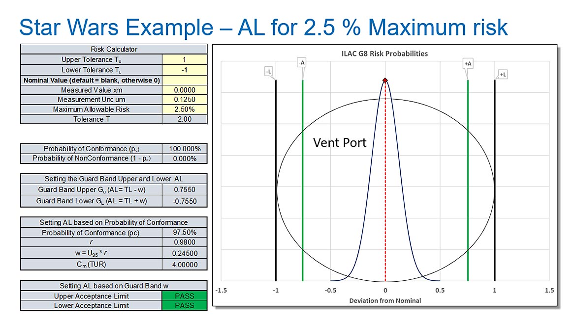
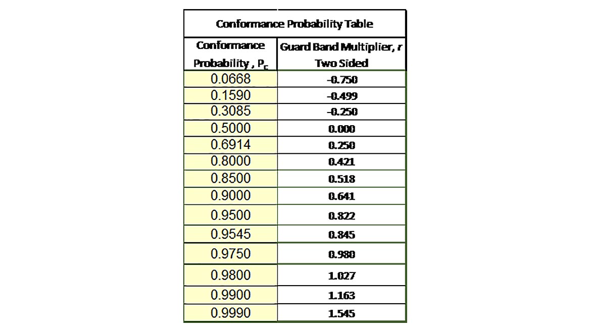
What we are calculating is our Conformance probability for 97.50 % Confidence. We calculate the Guardband Multiplier by using the formula in Excel of Norm.S.Inv(0.975)/2.
We then use this number of 0.845 as our GB Multiplier as follows.
For the Guardband upper limit, we have 1 – (GB Multiplier * Coverage Factor * Standard Measurement Uncertainty)
1 – (0.980 * (2 * 0.125)) = 0.7550
For the Guardband lower limit, we have -1 + (GB Multiplier * Coverage Factor *Standard Measurement Uncertainty)
-1 + (0.980 * (2 * 0.125)) = -0.7550
The formula can be simplified to Acceptance Limit = Tolerance Limit ± Guardband multiplier * Expanded Measurement Uncertainty.
ILAC-G8:09/2019 simply states, "Often the guardband is based on a multiple r of the expanded measurement uncertainty U where w=rU. For a binary decision rule, a measured value below the acceptance limit AL = TL – w is accepted." 1
Thus, if our measured value or shot is right at 0.7550, our risk will be limited to 2.5 %. If our X-wing takes the shot and the torpedo falls between the limits of ± 0.7550, there would be a 97.5 % chance that the shot would destroy the Death Star.
What if Luke takes the shot, and the measured value is 0.99?
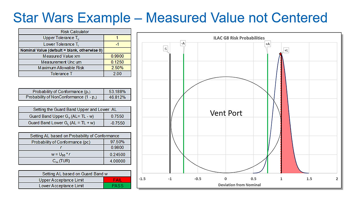
In this case, we can see that about 46.812 % of our 0.5-meter torpedo or 0.23406 meters of torpedo will hit the side of the vent, and the Death Star will not be destroyed.
Although this example uses a physical example of the torpedo either going into the hole or hitting the side of the vent port, the hope is it conveys the concept of specific risk.
Specific risk (also called bench-level risk) is based on a specific measurement result.
It triggers a response based on measurement data gathered during the test.
Depending on the method, it may be characterized by one or two probability distributions.
Any representation with only one probability distribution is always a specific risk method.
In our example, we used the size of the torpedo as our standard uncertainty of the calibration process, then multiplied that by a coverage factor of k = 2 to use as our Expanded Uncertainty of the calibration process.
Destroying The Death Star – Global Risk Example
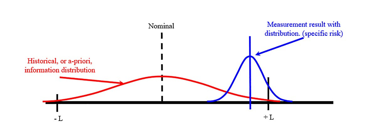
Global risk (also called process-level risk) is often based on a future measurement result.
It is used to ensure the acceptability of a documented measurement process.
It is based on expected or historical information and is usually characterized by two probability distributions.
If we look at the same example, we might say that the X-wing is not that much different from the T-16 skyhopper that he used to blast womp rats.
Using the fact that Luke was such a skilled shot, the best amongst all his friends on Beggar’s Canyon, we could use this a piori knowledge in a global risk scenario.
Based on Luke’s history, the historical context suggests that he will be able to hit the target.
One curve is our specific risk curve.
If the shot was measured at 0.99, there was a 46.812% chance the shot would not go in; however, this new knowledge, or curve, suggests, by using the law of averages, which the shot has a 99.11% chance of going in.
Say what now?
That’s more in line with how global risk works.
We are no longer controlling the quality of individual workpieces; we are controlling the average quality of workpieces. To control that average quality, we need to have the data.
In simplistic terms, End of Period Reliability is defined as the number of calibrations that meet acceptance criteria divided by the total number of calibrations.
Reliability Considerations may include:
- Reliability decreases with time after calibration
- How much testing is required to demonstrate Reliability with confidence?
- A priori knowledge of the M&TE
This formula to determine "In-Tolerance" Reliability from historical data is easy to replicate in Excel. The formula is Sample Size = ln(1-Confidence)/ln(Target Reliability).
When we use this formula for 95% EOPR at a 95% Confidence Interval, we need 59 samples with 0 failures or rejects as this will give us an estimation of our process.
Thus, if Luke successfully targeted 59 womp rats out of 59 shots, we would now have our reliability data and could start to use global risk models.
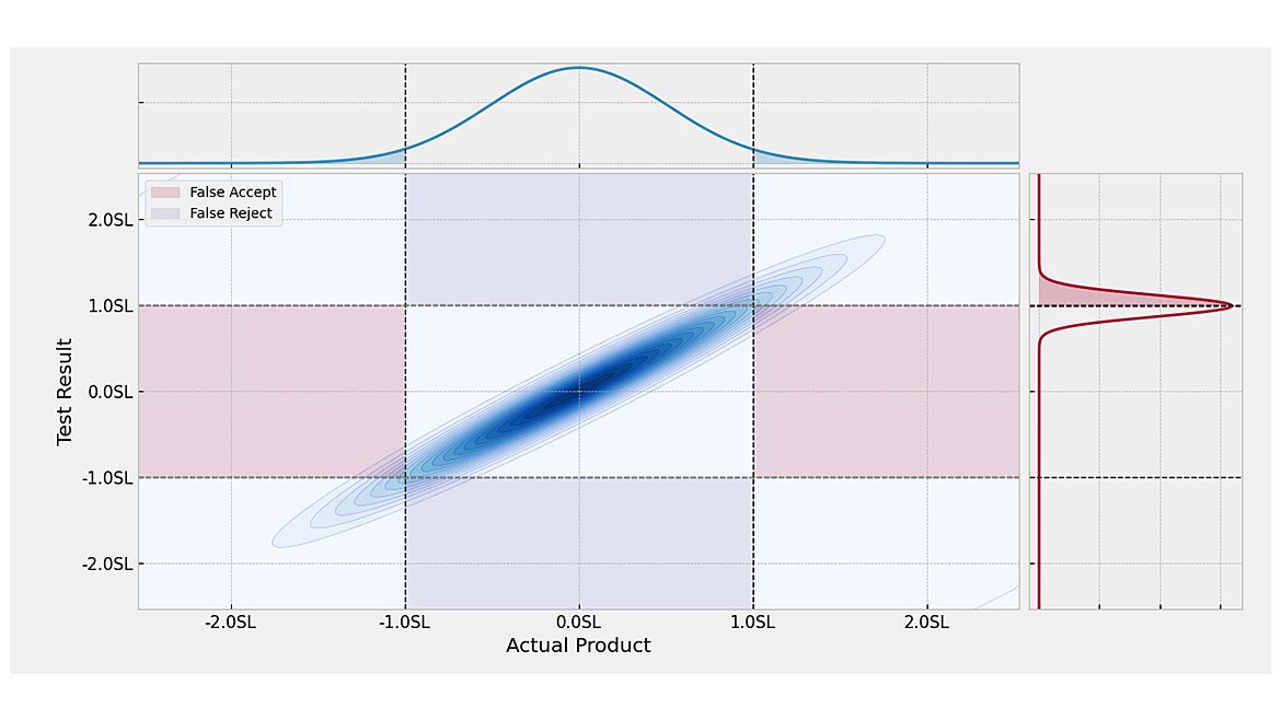
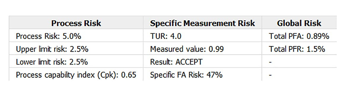
Setting this example up in Suncal shows our Specific Risk to be the same.
The global risk, however, shows a 0.89% chance we would say something is good when it is bad or a 1.5% chance, we would say something is bad that is good.
When using any risk model, the Expanded Measurement Uncertainty, including contributions for the Device Under Test, always determines the risk level or the acceptance zone.
If the risk is to be controlled to less than 2%, a 4.6:1 TUR can limit the risk Probability of False Accept Risk to less than 2%.
This is where effort needs to be made by the team that oversees what equipment to purchase to ensure the proper ratio is maintained.
For Instance, the example shows a 4:1 TUR ratio.
If equipment could be procured with a 10:1 TUR ratio, the total PFA would drop to 0.44%, and the PFR would drop to 0.47%.
This brings us to the following example of using global risk to manufacture a clone army.
Star Wars Global Risk: Building A Clone Army
We want to build an army of clones to defeat the Rebellion.
The optimum height is 70 inches ± 2 inches to fit our clones with the same gear and maximize cloning efficiencies.
Our measurement system has a TUR of 8:1, meaning our Calibration Process Uncertainty is 0.25 inches.
The question becomes, what is the probability of saying a clone conforms to the specification when it does not?
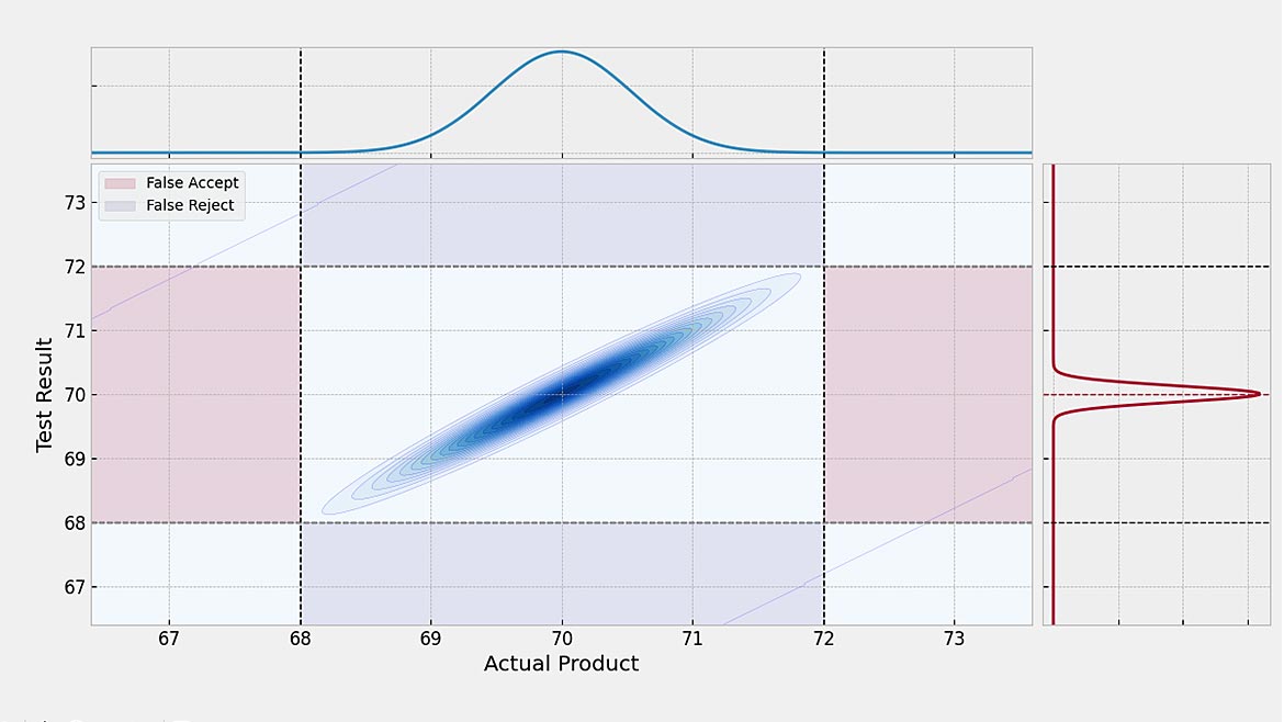
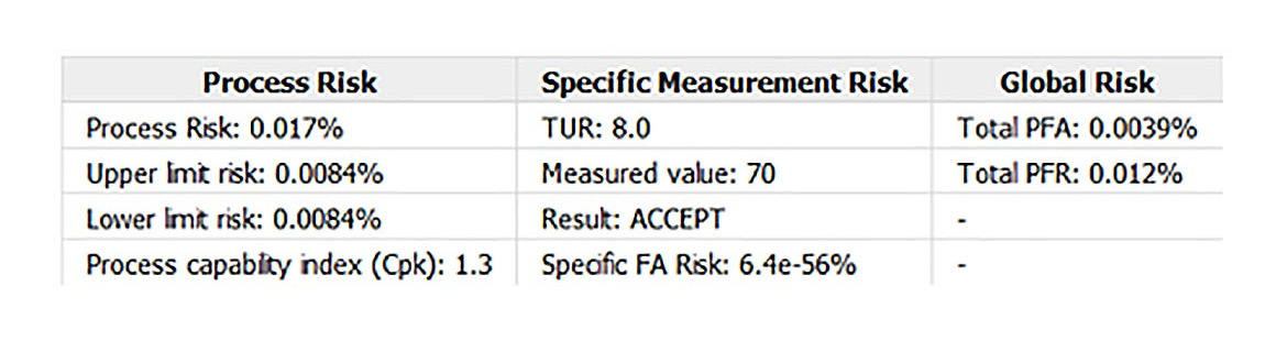
Using the Suncal software, we key in our lower specification of 68, our upper specification of 72, and 0.125 as our Expanded Uncertainty of the calibration process.
When using these values, we find about 0.0039% or 3.9 per million are expected to be said to be in conformance when they are not.
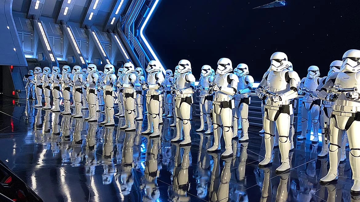
This translates to about 1 out of every 500,000 being too tall and thus demonstrated in Star Wars Episode IV: A New Hope by a stormtrooper hitting their head as they were taller than their counterparts.
Shifting the focus toward design, particularly regarding headgear, recalls the importance of Luke’s experience when he dons the Storm Trooper gear and exclaims, "I can’t see a thing." This underscores the need to concentrate on essential aspects when designing and testing models based on our risk assessments.
Consider this: if we invest heavily in building an army of clones but equip them with armor that impairs their vision, can we realistically expect to rule the galaxy?
As basic as it may sound, such oversights occur daily in manufacturing and measurement.
Numerous organizations overlook the crux of the matter: understanding the right requirements and ensuring that the products they design conform precisely to those requirements and specifications.
Star Wars Risk Conclusion
Using Star Wars as an example highlights the cost-saving potential of managing measurement uncertainty in global and specific risk scenarios. ASME B89.7.4.1-2005 effectively delineates these risk levels.
In ASME B89.7.4.1-2005, specific risk mitigation equates to "controlling the quality of individual workpieces," while program-level risk strategies involve "controlling the overall quality of workpieces." [i]
Specific risk is akin to immediate financial liability at the moment of measurement. This concept aligns with using specific risk or bench-level measurements for standards that are vital in precise measurements, similar to the precision required to fire a proton torpedo into the Death Star’s vent port.
In manufacturing, the focus often shifts to managing average quality, where program-level risk pertains to the average likelihood of making incorrect acceptance decisions based on historical data.
In both cases, investing in equipment that reduces the Test Uncertainty Ratio offers substantial cost savings by minimizing rework and ensuring more accurate acceptance and rejection decisions.
Resources:
- ILAC G8:2019 "Guidelines on Decision Rules and Statements of Conformity."
- ASME B89.7.4.1-2005 "Measurement Uncertainty and Conformance Testing: Risk Analysis"
Looking for a reprint of this article?
From high-res PDFs to custom plaques, order your copy today!


