Portable phased array ultrasonic testing systems hit the market nearly 20 years ago, and today the latest generation of these tools delivers better amplitude resolution, faster data acquisition rates, and advanced data analysis in a single easy-to-handle package.

Their computing power also gives NDT technicians access to data analysis techniques—and inspection opportunities—that once seemed out of reach.

One of these is Full Matrix Capture (FMC), a data acquisition strategy that leverages phased array UT to capture every possible transmit-receive combination for a given ultrasonic phased array transducer. It can increase the reliability of inspections and reduce the need for costly and time-consuming re-scans.

How it Works

Phased array UT systems use probes with multiple elements (typically from 16 to 64) that are excited by a computer in a highly controlled manner, using a specific delay law and, after reception, the contribution of each element is summed to produce one A-Scan. The phased-array UT instrument can produce a focused beam of ultrasound that can also have different steering angles. This can simplify and improve the inspection of complex geometries and dissimilar materials, which are challenging to inspect because of the varying acoustic properties you’ll encounter.

The important thing to remember is that with phased array UT, a single pulse and single reception produce a single A-scan. With FMC, each array element in a probe is sequentially used as a single emitter while all array elements are used as receivers. By capturing and storing A-scan signals from every transmitter-receiver pair in the array, it’s possible to generate UT imaging for any given focal law/beam (aperture, refracted/skew angles, focusing position) and to apply the latest post-processing algorithms today or as they improve in the future. The set of FMC data can be processed multiple times to produce different results, using different reconstruction parameters.

One example involves the Total Focusing Method (TFM), an advanced processing algorithm that uses FMC-collected data to generate a frame of pixels where each pixel is computed using a dedicated focused focal law. This results in one focal point per pixel; in theory, every pixel is perfectly focused. With the right combination of hardware and software, FMC and TFM together are a powerful tool for processing and reconstructing data for defect characterization.

Scope and Scale

To understand the scope of data acquired during FMC, consider this example:

A probe has the number n elements. It therefore must be pulsed n times, or once per element, which implies that the acoustic travel time of an ultrasound pulse occurs n times. Because an elementary A-Scan is digitalized for each pulse n, the total number of elementary A-Scans gathered after the full firing cycle is n2.

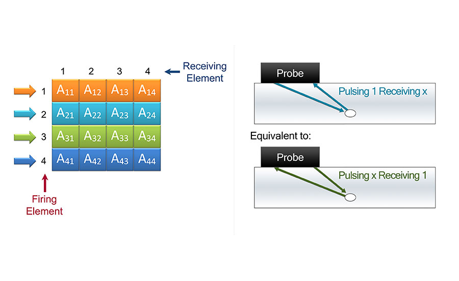
Figure A.

Here’s how data acquisition will scale when n is 16, 32, and 64 elements:

• 16-element probe: Probe pulsed 16 times, 256 elementary A-Scans gathered
• 32-element probe: Probe pulsed 32 times, 1,024 elementary A-Scans gathered
• 64-element probe: Probe pulsed 64 times, 4,096 elementary A-Scans gathered

The number of scans gathered is a factor in both storing the data and the ability to regenerate images later.

Even if you don’t understand all the technical details, here’s an explanation that should convey why file size is such a challenge with FMC.

In its typical configuration using today’s technology, FMC is performed with a 64-element probe in order to enhance aperture size, beam-forming capability, and focusing power. A typical elementary A-Scan length can be around 80 µs and each one must have a sufficient time base so the maximum applied delay law plus depth of coverage is fully contained. This usually translates to an A-scan with 8,192 samples, 2 bytes per sample (12 to 16 bits amplitude).

Therefore, the storage required for a single FMC probe location is 64 MB: 4096 * 8192 * 2 (elementary A-scan * sample count * byte count). This file size is for each probe location along a scan line.

The large amount of storage required for FMC (up to 64 MB of data for a 64-element probe) is subject to further scale factoring. To achieve sufficient acquisition speed, the instrument data throughput has to be very high. For example, to achieve 30 Hz requires data throughput of 1.8 Gigabyte per second (64 MB * 30 Hz). So scanning a typical 12-inch pipe with typical resolution would produce very large files for an NDT application: (12 inches * 3.1416/0.039-inch scan resolution) * 64 MB = 60 GB.

Managing File Sizes

While the hardware and software used for FMC data acquisition need to be able to handle a substantial amount of A-Scan data, file sizes and data accumulation can be reduced or at least made more manageable.

Consider the basics of FMC firing and receiving. The description of element combinations can be represented in a firing matrix. Rows represent firing elements and columns represent receiving elements.

In the firing matrix shown in Figure A, there is pair of combinations that have the equivalent ultrasound path and characteristics: A21 is equivalent in path and signal to A12, and A41 is equivalent in path and signal to A14.

Figure B.

Half Matrix Capture (HMC) is a principle that’s intended to factor out these identical paths. By applying HMC, the number of A-Scans required drops from n2 to n (n+1)/2. For each equivalent pair, only one combination of elements is kept which reduces the amount of data required by nearly one-half, as in Figure B.

How to Use FMC Data

Due to the large amount of data produced per second, there are typically two ways to handle FMC data today:

1. Use and discard: Some instruments are using FMC data for a single probe location within the instrument, and processing it with dedicated high-speed hardware. The FMC data is processed and sent to the software for viewing, and then discarded to preserve usable space and speed.

2. Transfer, keep, and reuse: Some instruments also support storage of FMC data. Transferring data from the instrument to a computer requires the most efficient data link available. Due to its size, FMC data consumes hard disk space but storing raw A-scan signals means you can analyze it with different sets of reconstruction parameters at virtually any time.

The FMC technique continues to develop as hardware and software engineers focus on systems that support a high number of A-Scans per acquisition point, provide a very high data transfer rate, can handle large data files, and produce very high signal quality. It remains an advanced technique, and one that more technicians should understand in order to maximize the capabilities of their tools.