I often hear, “How accurate can this be measured using CT?” For CT accuracy and precision should be considered together. For accuracy versus precision, picture a target.

On the upper left the shots are scattered, relative to the lower right, so precision and accuracy are low. The top right shows a “good grouping,” all close to each other but not close to the center. On the lower left all are around the center, some scattered inside the second ring showing high accuracy but low precision.

In order to further answer the questions of accuracy, let’s establish some additional definitions:

1. Tolerance refers to the difference between the upper (maximum) limit and lower (minimum) limit of a dimension. In other words, tolerance is the maximum permissible variation in a dimension.
2. Uncertainty of measurement is a value of how much the real value is likely to be at a certain confidence level. It is common to accept a confidence level of 95 percent.
3. Voxel size is the size of the smallest information created by a CT unit. This is easy to determine by simply dividing the field of view by the number of voxels in the same direction in space.
4. Contrast or Density Resolution is the property of a CT unit of recognizable reproducing objects of low contrast or density relative to homogeneous surroundings.
5. Spatial Resolution is the property of a CT unit of recognizable reproducing objects lying close to each other as separated from their surroundings.
6. Structural Resolution is smallest structure that can still be measured dimensionally.
7. Error describes the system performance and is the deviation from a known measurement under specific conditions. A system is specified to perform within the limits defined as maximum permissible error MPE. There may be multiple different specifications for one system. The error is not the same as uncertainty of measurement.

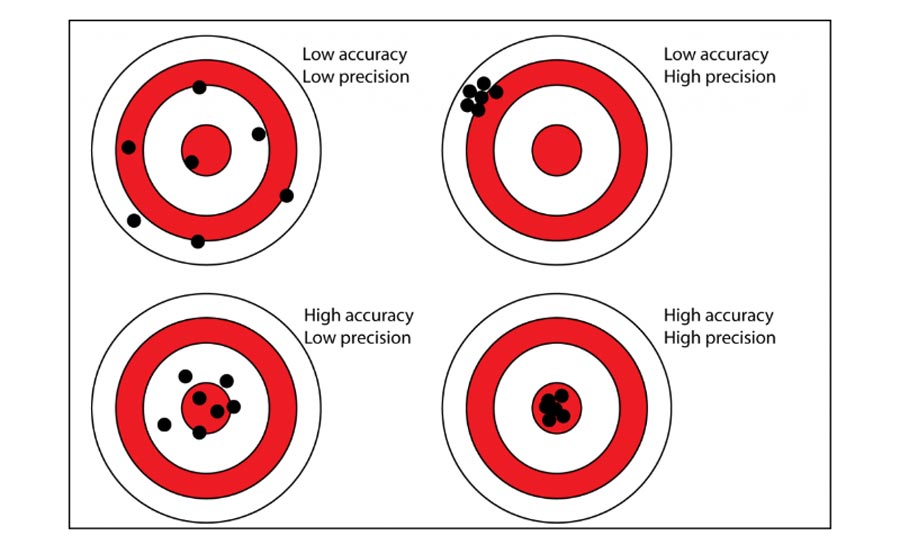
Fig. 1 – Accuracy and precision

From Voxels to Surfaces

In CT, X-ray photons emitted from an X-ray tube travel through the object and hit a detector which senses the dose at each pixel of the detector area creating digital images while the object is rotated. Reconstruction software calculates virtual slices based on the dose at each location from different angles creating a tomogram. Each pixel in the tomogram represents a density of material, called voxel (volume pixel).

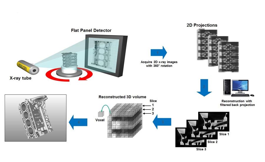
Fig. 2 Computed Tomography (CT) Principle

To measure features, it is necessary to give the object a surface. This is done by looking at an area of material and area of air. The value in the middle is used as the threshold (ISO 50 method) to set points on the surface.

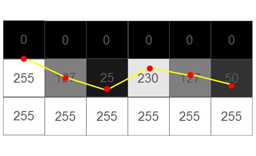
The red point most left is between the black voxel (gray value 0) and the white one below (gray value 255). For simplicity, the example only shows the point being place in vertical direction. In real life this is done in all three directions. The next one to the right shows a voxel of 127 which places the surface right in the middle of the voxel. With gray values closer to black and white the surface moves accordingly to that direction.

Under ideal conditions, surface accuracy would be 1/256 of the voxel size. That assumes the area coverage of the material creates a signal (gray value) change proportional to the area covered. In reality, the scan data are 100 percent perfect due to multiple physical effects like scatter radiation, pixel noise and approximation in the reconstruction algorithms. A good rule of thumb is to use 1/10 of the voxel size is the accuracy of the surface on a decent CT scan. Many unknowns make it difficult to state a hard number. Fortunately, there are ways to find the uncertainty of measurement and standards that can be used.

Uncertainty of Measurement

The first standard is the GUM (Guide to the expression of uncertainty in measurement, JCGM 100:2008). This standard is a general guide and can be applied to any measurement and unit. The standard was mainly written by mathematicians, so you see formulae and hard-to-understand verbiage. However, there are more hands-on standards with GUM built in and we don’t have to understand everything in GUM down to the smallest detail.

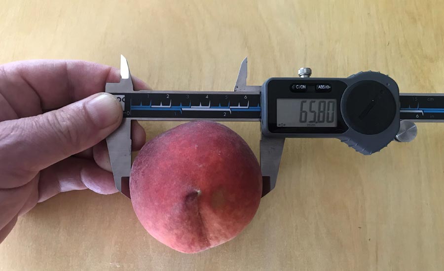
Fig. 4 Measurement of a peach and a cobalt square

The first step is modeling the process to understand how the measurement results are distributed. In most cases, assume the measurements are distributed under a bell curve and huddle around the mean value.

The guide gives two ways to proceed: Type A or Type B. Type B is based on experience and previous data. If you have done Type A many times you can use your judgement to come up with a number.

For a new application, use Type A. Measure one or more objects of the same type and analyze the observations. To illustrate the object’s impact, I measured a peach and a cobalt square for machine tools. They are totally different; the peach is soft and hard to measure the same spot. I tried to measure the same distance with same force using a digital caliper. The cobalt square was measured with the same digital caliper at the same location. I performed 20 measurements on each.

The difference in deviation suggests the object itself has an impact on the uncertainty of measurement. The peach’s standard deviation was 234 µm and cobalt square’s only 3.66 µ. Both objects were measured at approximately the same time and temperature.

The next step under GUM is determining “Combined Standard Uncertainty” (uc), which can be measured by:

• Standard deviation over all measurements divided by SQRT
• Standard deviation of mean values

In our two-measurement series we measured each object 20 times, choosing the first method to calculate combined standard uncertainty.

Confidence level is part of uncertainty, that’s where the coverage factor comes into play. This factor k generally ranges from 2 to 3. In practice:

• k=2 confidence level 95%
• k=3 confidence level 99%

The expended uncertainty U is the product of the standard uncertainty uc and k.

This experiment shows measurement equipment only partly contributes to uncertainty of measurement. The standard is a reliable method to produce an objective “hard” number for the uncertainty of measurement.

CT System Performance:

DIN EN ISO 10360 Geometrical product specification is the gold standard for 3D measurement equipment. It compares different equipment and defines clear understanding of when a system is within the specification. There two series of standards under VDI/VDE applicable for CT: VDI/VDE 2617 Accuracy of coordinate measuring machines and VDI/VDE 2630 Computed tomography in dimensional measurement.

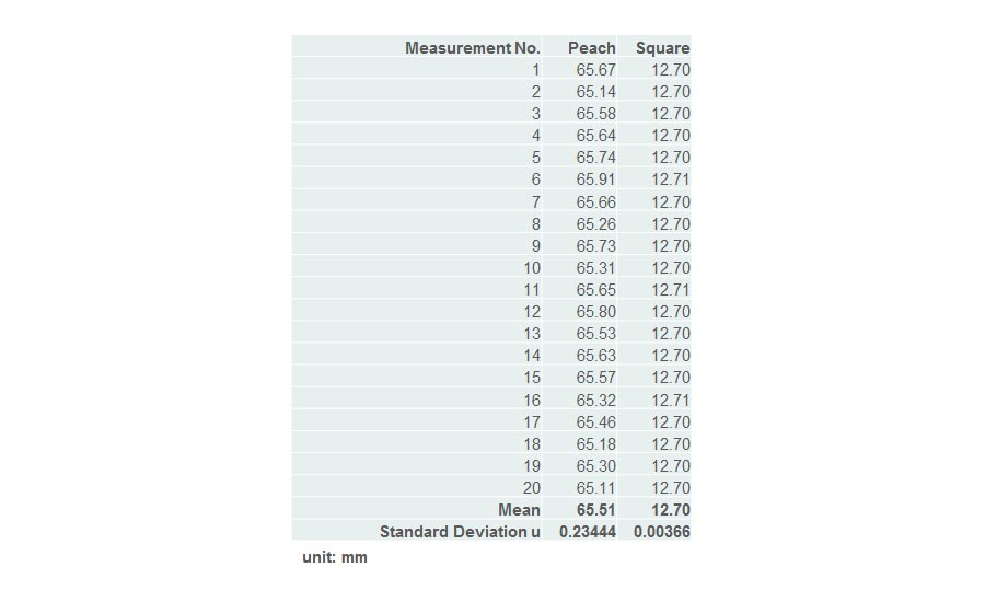
Fig. 5 Measurement Experiment, mean value and standard deviation

The two standards cross over with VDI/VDE 2617 part 13 and VDI/VDE 2630 part 1.3, providing a guideline for applying DIN EN ISO 10360 for coordinate measurement machines with CT sensors. VDI/VDE 2630 part 1.3 provides three guidelines:

• Fundamentals: Definitions of characteristics (probing error, length measurement error, size and form error) and limits
• Acceptance test: How to determine a CT system meets the limits of the characteristics
• Monitoring: Long-term compliance with the characteristics

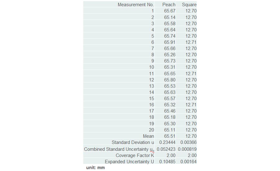
Fig. 6 Measurement Experiment to determine Expanded Uncertainty U

It recommends using spheres or spherical caps made of “suitable material,” normally defined by the manufacturer. Ruby is commonly used since high-quality ruby spheres are commercially available and thermally stable. The spheres by themselves allow you to determine probing error form and size. Placing several spheres in the scan volume makes it possible to measure the sphere distance accurately with minimal impact related to surface determination as sphere centers are relatively stable. With several ruby spheres, different distances can be measured. This test specimen is easily calibrated and traceable to NIST.

The results are compared to manufacturers’ limits and a compliance report is created.

Repeatability and Suitability

Quality standards like ISO 16949 mandate statistical analysis of measurement processes. Factors that influence measurement results are commonly shown in a fishbone.

When performing the analysis, the process should include all possible variables. For example, temperature should vary in a realistic range. If temperature impacts the result, the process should not be analyzed at only one temperature if in the real process the temperature changes.

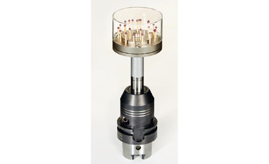
Fig. 7 Ruby sphere specimen

Compare tolerance and uncertainty to decide if the process is suitable for the application. There are a variety of industry standards, however Part 2.1 of VDI/VDE 2630 was developed for users of industrial CT systems. Part 1.3 helps buyers and sellers agree when and how a CT system is performing to meet the specified characteristics. The specified MPEs (maximum permissible error) have nothing to do with a specific application. That’s where part 2.1 serves to determine the uncertainty of measurement of specific features and to give the user help deciding if the process is suitable for the required tolerance of that feature. It is based on GUM and traceable.

The core to determine is this formula for the expanded uncertainty of measurement.

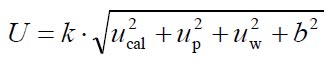
U: Expanded uncertainty of measurement

k:  coverage factor (2 for 95%)

u_cal: uncertainty of the calibration measurement

u_p: standard uncertainty of the process

u_w: uncertainty of the workpiece

b: systematic deviation

To solve the equation, run several measurements. The standard suggests having one sample calibrated with a method that is more accurate, normally in a certified lab with a highly accurate CMM. The lab provides the uncertainty of the measurement (ucal). This calibrated sample would need to be measured 20 times (the suggested number covering most variations of CT scanning). The standard uncertainty of the process with n being the number of measurements is calculated.

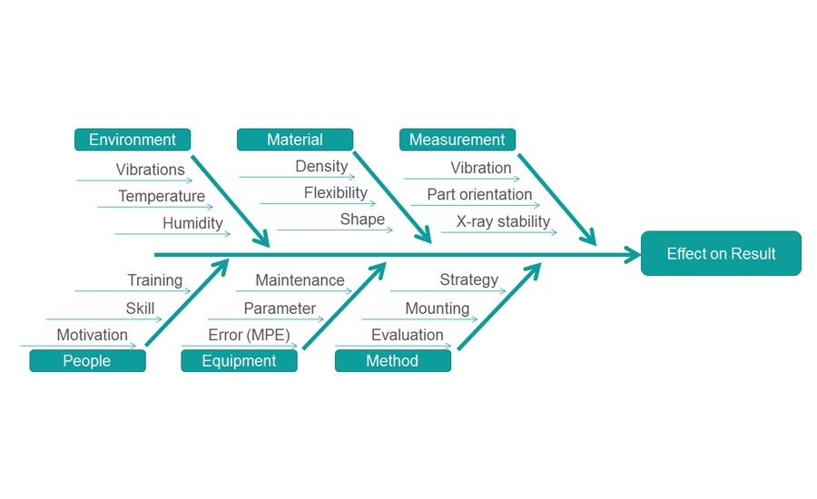
Fig. 8 Fishbone diagram for measurement effects

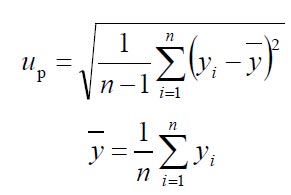
Fig. 10 Standard uncertainty of the process up

It is also suggested to measure multiple samples not only the one that is calibrated. Part 2.1 suggests four samples including the one that is calibrated.

The standard uncertainty of the total process would take all four sample measurement series into account and up be calculated with this formula:

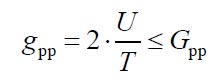
Fig.11 Standard uncertainty of the total process up

Now that we have up, consider uw. It’s important to cover all variations possible during the measurement process. If measurement changes are expected, for example temperature, the uncertainty resulting in this must be calculated. Thermal expansion is easy to calculate. If the multiple samples were used for up the uw and all workpiece relevant variations are cover this part can be set to zero.

“b” is the systematic deviation and basically the difference between the mean of all calibrated sample measurements and value of the calibration measurement.

Finally, determine uncertainty of measurement in relation to tolerance. Part 2.1 suggests Gpp between 0.2 and 0.4 following this formula:    

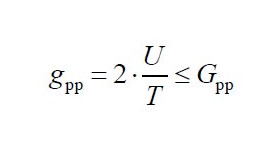
Fig. 12 Double sided tolerance

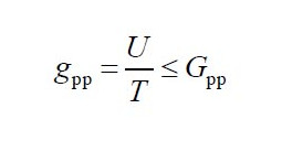
Fig. 13 Single sided tolerance

Single-sided means there is a tolerance mandating a value not being greater than x or smaller than y. Double-sided is a tolerance like +/- 0.01mm, with an upper and lower limit.

So, now you can see why my answer to the general question regarding accuracy of CT is not simple. However, if you take time to understand these definitions, standards and testing methods, you’ll be able to determine the accuracy of CT in your specific application. My suggestion is to work with a CT system provider if you’re not certain about the processes or accuracy to learn how to effectively and efficiently obtain the best results. NDT