Vision & Sensors | Lenses
Understanding the Key Factors in Microscope Objective Performance

Image Source: gorodenkoff / iStock / Getty Images Plus via Getty Images
To no surprise, a microscope objective is the most important imaging component of an optical microscope. A microscope objective is a multi-lens assembly that focuses light from an object and forms an intermediate image that is projected onto a sensor or magnified by an eyepiece. There are two types of microscope objectives: finite and infinite conjugate. Finite conjugate objectives work like any other lens where an image is formed when an object is located at a finite distance beyond the front focal point. On the other hand, infinite conjugate objectives require additional optics, often referred to as a tube lens, to focus the ray bundles to form an image. This objective design allows for the introduction of other optics such as filters, polarizers, and beamsplitters, making it a popular choice for high magnification imaging systems.
Besides deciding on the type of objective, imaging system designers often consider the magnification, numerical aperture (NA), and cost options available to make their decision. Numerical aperture often has the biggest influence in a decision between two objectives with the same magnification as NA is believed to directly equal to performance. However, NA does not tell the whole story about a microscope objective’s imaging performance. This article will go over what defines a microscope objective’s performance and how this can be applied when developing high-magnification imaging systems.
What is Numerical Aperture?
NA is an important specification to define for a microscope objective because it describes the objective’s throughput, or ability to gather light, at a fixed working distance. The equation below is the first-order equation used to calculate NA. An objective’s throughput is limited by the angle θ and as the angle decreases, the NA will also decrease. This equation is useful for understanding NA on-axis as it only considers what is happening at the center of the field.
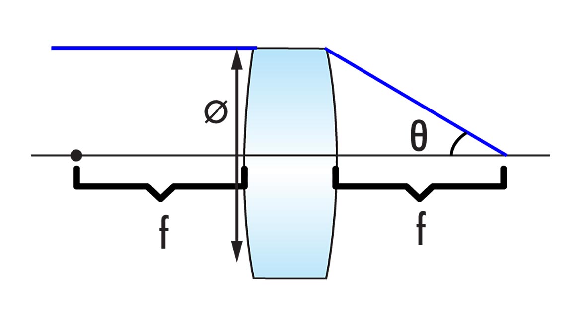
NA=n*sin(θ) [1]
n: refractive index of imaging medium
θ: one-half of the objective’s opening angle
The NA is often assumed to describe an objective’s resolving power; however, this is not an accurate assumption. It is a great proxy for understanding the resolving power of an objective, but does not consider field changes for off-axis performance. Equation 2 below relates the resolution of an imaging system to NA. This equation defines the minimum separation between two point sources of light that an imaging system can resolve at a certain contrast level. Similar to equation 1, this equation is only useful for assessing system resolution in image space and does not consider off-axis fields.
Resolution= λ/(2*NA) [2]
λ = wavelength
What Affects Numerical Aperture?
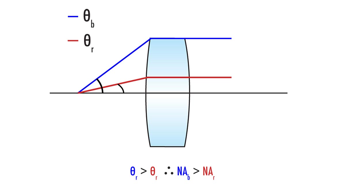
Aperture size
When looking at what can affect the NA of a lens, the first thing that comes to mind is the aperture of a lens. Lenses with large apertures will have larger angles for increase light collection through the system. As observed in Figure X below, angle θb will yield a larger NA lens compared to a smaller aperture lens with angle θr. The larger aperture lens will have a high throughput and as a result, will be able to resolve smaller features and have an increased brightness compared to a smaller aperture lens.
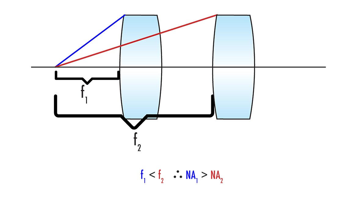
Focal length
Focal length also affects how much light a lens can collect. When comparing two lenses of the same diameter like in Figure X., the lens with a longer focal length f2 will collect less light. This is because the angle θ decreases as the focal length of a lens increases. As a consequence, the NA of the longer focal length lens is smaller and is not as efficient in light collection compared to a shorter focal length lens.
Departure from Theoretical
Vision & Sensors
A Quality Special Section
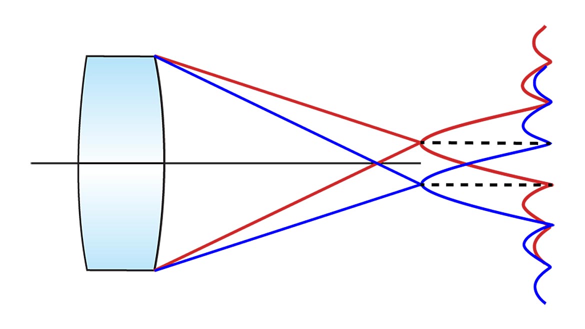
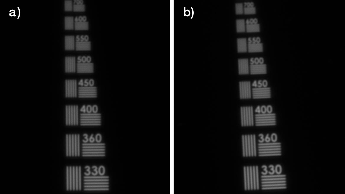
To understand the nuances of NA, two 5X objectives with a NA of 0.14 where compared for their imaging performance with a high-resolution USAF microscopy target. The evaluation criteria for being able to resolve a given frequency was a contrast value above 20%, which is a standard commonly used to evaluate an imaging lens. Their performance was looked at on-axis and off-axis to compare the theoretically calculated resolution to actual performance. Using equation 2, the diffraction limited performance is calculated to be 2.1 µm, or 238 lp/mm when converted to frequency. The figure below shows that they can resolve above the diffraction limit frequency with high contrast when looking at the target on-axis.
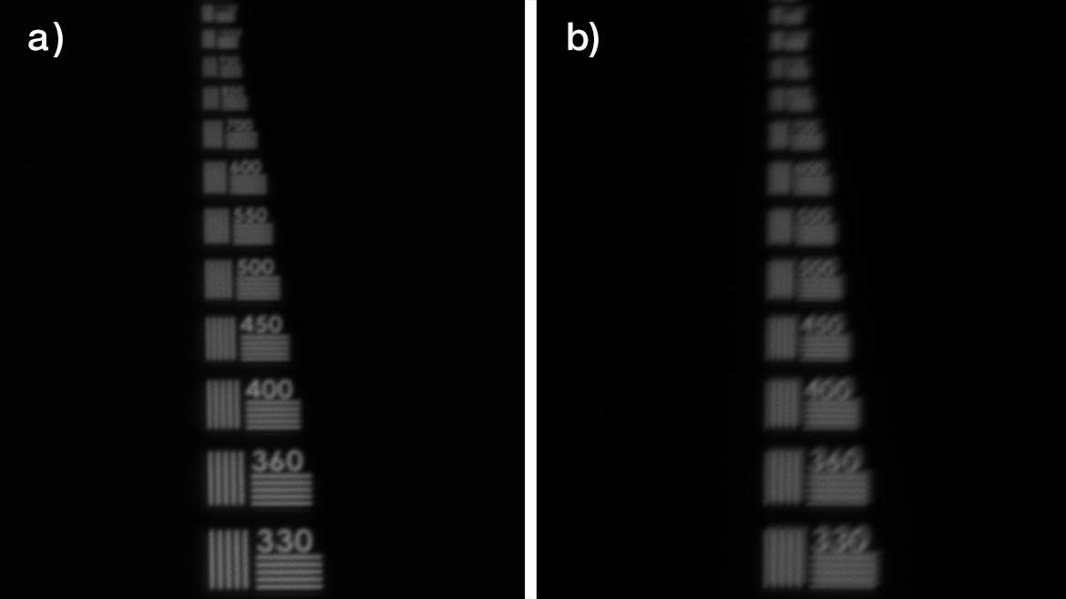
The figure below shows the off-axis performance of the objectives. There is a significant decrease in contrast for one of the objectives compared to the other as it can no longer resolve the same frequencies off-axis that it could on-axis. While these objectives look identical when comparing their specifications, there is a clear difference in resolution off-axis. This indicates that NA is not the defining factor for the performance of an objective.
There are several contributing factors as to why the theoretical calculated diffraction limited performance doesn’t accurately match real-world data. The first being that the calculation only uses a single wavelength which isn’t representative when a broadband light source is used. Shorter wavelengths will yield a higher resolution compared to longer wavelengths in the visible spectrum. Another factor is that modern machine vision cameras have smaller pixels. Smaller pixels allow a lens to more accurately distinguish the separation between two small objects that are very close together. As a result, the lens will be able to resolve smaller features than the theoretical diffraction limit. Finally, tolerances during the manufacturing and assembly of microscope objectives can impact performance and are not considered in the theoretical calculation.
Application Example
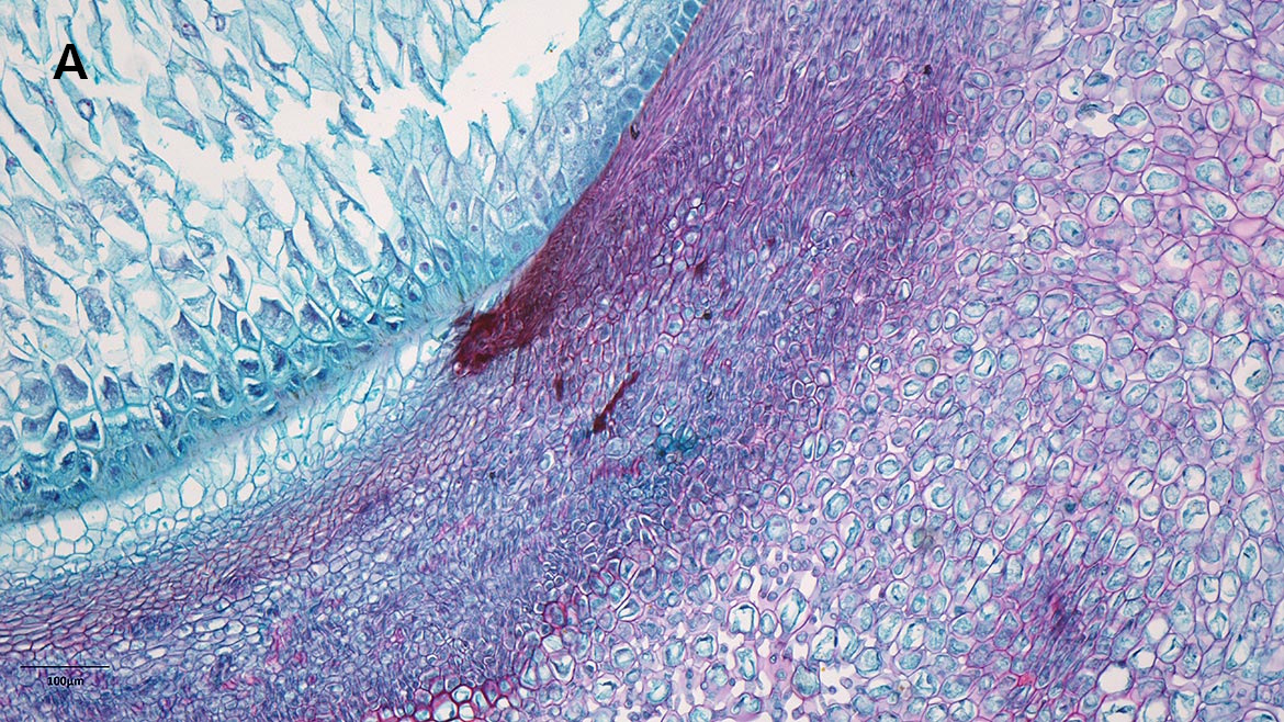
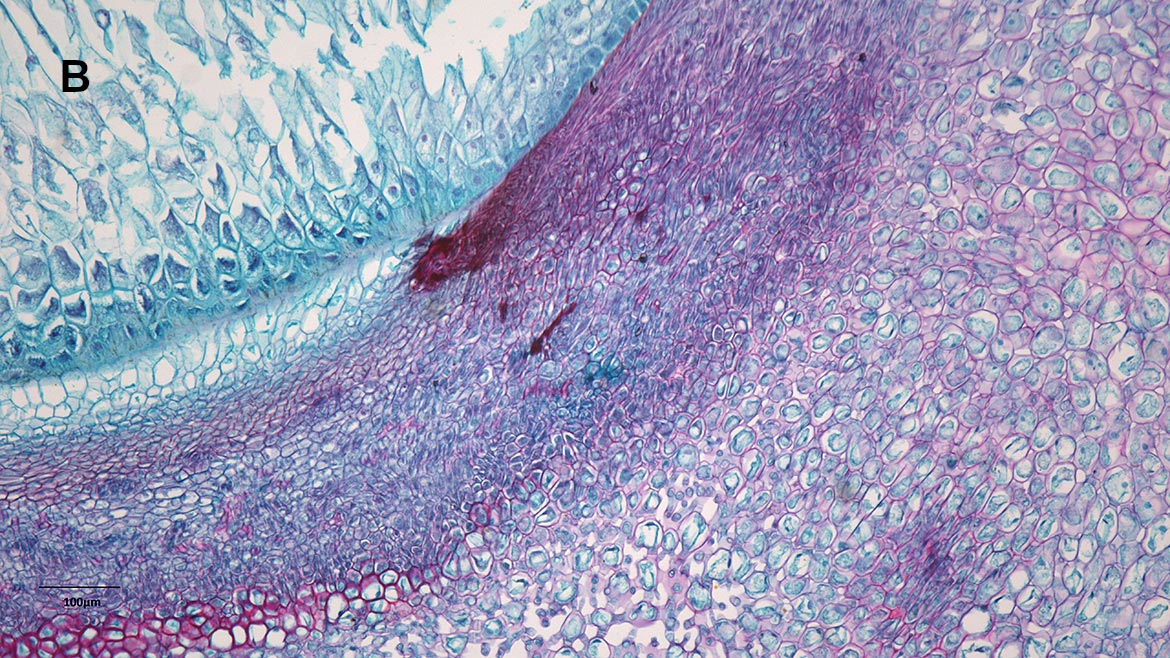
Maintaining performance off-axis is especially important for life science applications like microscopy and high-throughput imaging. In these applications, it is critical that information can be extracted from the entire image without any loss information. Using a microscope objective that maintains performance off-axis can ensure the imaging system produces reliable data. Below are images taken with 10X microscope objectives that have the same NA of 0.28. When looking at the off-axis performance, it is clear that one objective does not hold performance compared to the other. Both objectives are also considered to be Plan, which means they meet the minimum criteria required by ISO 19012-1 for flatness of the image field. While Plan is an important specification when selecting an objective, it also does not tell the whole story in terms of performance since there is only a minimum requirement of image flatness and not a standard value. This highlights the importance of testing each objective independently rather than comparing specifications.


Conclusion
When designing a high magnification imaging system, it is important not to compare objectives just based on their specifications. Many specifications only describe what happens on-axis and don’t consider performance across the entire field. Wavelength, aperture, focal length, and manufacturing/assembly tolerances all affect an objective’s performance and are not account for in specifications like NA and image flatness. Therefore, it’s important to evaluate an objective’s performance before implementing it in an imaging system to determine if it can resolve the necessary details across the entire field.
Looking for a reprint of this article?
From high-res PDFs to custom plaques, order your copy today!


