✕

Machine vision acquires images and reliably creates decisions and information from them on an automated basis. This article is about the “middle stage” of that process which is image analysis. Volumes have been written on this; the article seeks to provide a brief practical overview of some of the common software tools applied to images during typical machine vision solution design. It also strives to follow the advice of “if you can’t explain it simply, you don’t know it well enough” in its presentation.

The run-time machine vision process starts with acquisition of an image which provides reliable contrast of the type needed to enable the intended image analysis. Accomplishing this requires designing the illumination, the imaging, and the geometry and interaction between them and the workpiece. Some view this as “lighting up” the workpiece; it’s much more than that; we call it the physics part of the solution. Shortcomings in this process should be resolved rather than relying on image analysis to try to compensate for them.

For certain less typical types of imaging, the earliest stages might consist of putting together 1D line scan images to create a 2D image. Other transformations code an attribute other brightness into the pixel values of “grayscale” image. Examples of this are “depth” in a depth map image derived from a 3D point cloud or a color attribute derived from a color image.

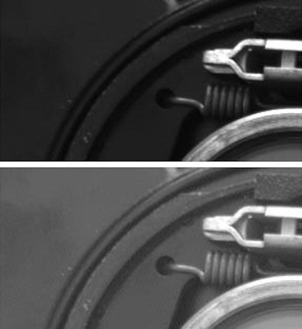
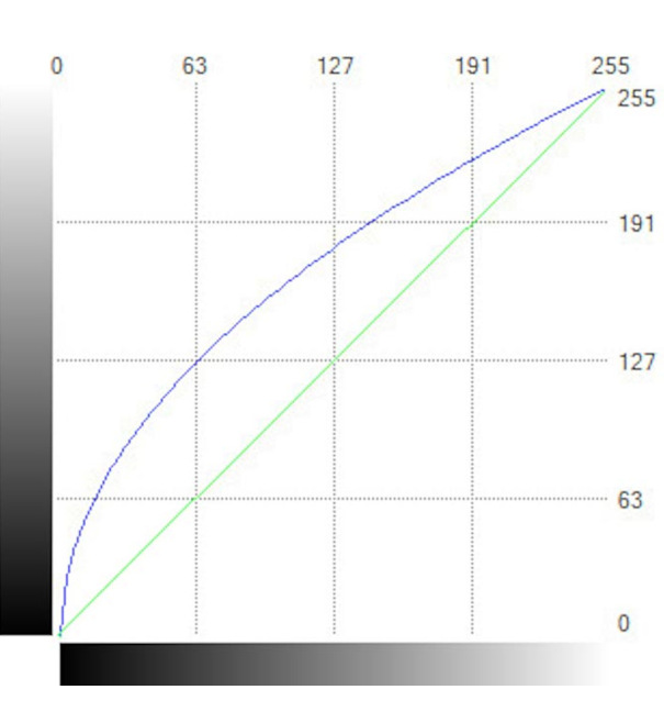
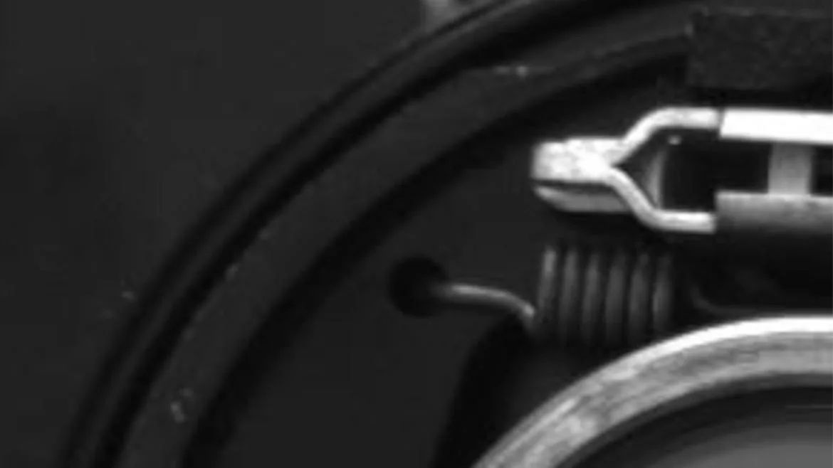
Early stages of image analysis may involve filters and similar tools which transform the entire image to enable or optimize the later stages. One of the simplest of these is a lookup table tool which creates an output value for each pixel based only on its input value (a distinction from a filter where the output value of each pixel is also influenced by its neighbors). This is most commonly used to increase contrast in one area of the gray scale. In figure 1 a “square root” lookup table is applied to the shown portion of a brake assembly in the upper half of the figure to provide greater contrast to the features in the dark areas shown in the lower half. The math of this transformation is illustrated in figure 2. The horizontal axis represents in input gray scale level and the vertical axis represents the transformed output value for that pixel. For 8-bit gray scale, the maximum for each axis must be 255, pure white. The green drawn “x=y” straight line graph would represent “no change”, and the blue curve represents the change applied.

Most tools that transform entire images or image sections are filters where the output value of a pixel is also affected by its immediate neighbors. Some common uses of filters in machine vision are using Sobel, Laplacian or Canny filters to emphasize or extract edges and mean, median, dilation, erosion, opening, and closing filters to remove small unwanted objects or texture.

Defining regions of interest is ubiquitous in machine vision. Examples of this are specifying an area for search or operation, or drawing a probe at a desired place to take a measurement. Some architectures allow objects found via image analysis to themselves be used as areas of interest.

A common task of machine vision image processing is separating an object from its surroundings. The most common tool for this is thresholding where it is separated based on differences in gray level. Areas that are darker or lighter than a specified grayscale value are extracted for subsequent processing. Again “gray level” may actually be other attributes mapped to the pixel such as 3D depth or color components.

One of the most common and wide-ranging image analysis tasks is presence detection which includes verifying the presence of things that are required to be there and detecting the presence of things that are not supposed to be there. An example of the former is to verify that a correct part is installed in a correct location during an assembly process. A typical approach is for the processing to look at the place where the object is required to be, turn what it found there into an object for further analysis, and then analyze it to the degree needed to assure that it is the correct part and properly placed. The same concept may be used for robot guidance where location and orientation measurements of found objects are passed off to a robot so that it may properly grasp the product.

An example of detecting the presence of things that are not supposed to be there is surface analysis. Defects are separated via thresholding and then some measurements are taken on them to determine their severity. In this area, overall measurements (such as length, width, area) of the items found are taken; this is distinct from gauging where measurements at certain points are taken. A common tool name that bundles some of these functions is sometimes called “blob analysis.”

Deep learning/“AI”/neural net machine vision image analysis has made rapid advances in recent years (see The Place for Deep Learning in Industrial Machine Vision). Some forms that operate on extracted parameters go back decades, but the large advances in recent years have been on deep learning based analysis of whole images. The most common results of these tools are detection of objects and classification of them into classes. A class can be as simple as “pass” or “fail,” a type of part, or characters of the alphabet for OCR purposes.

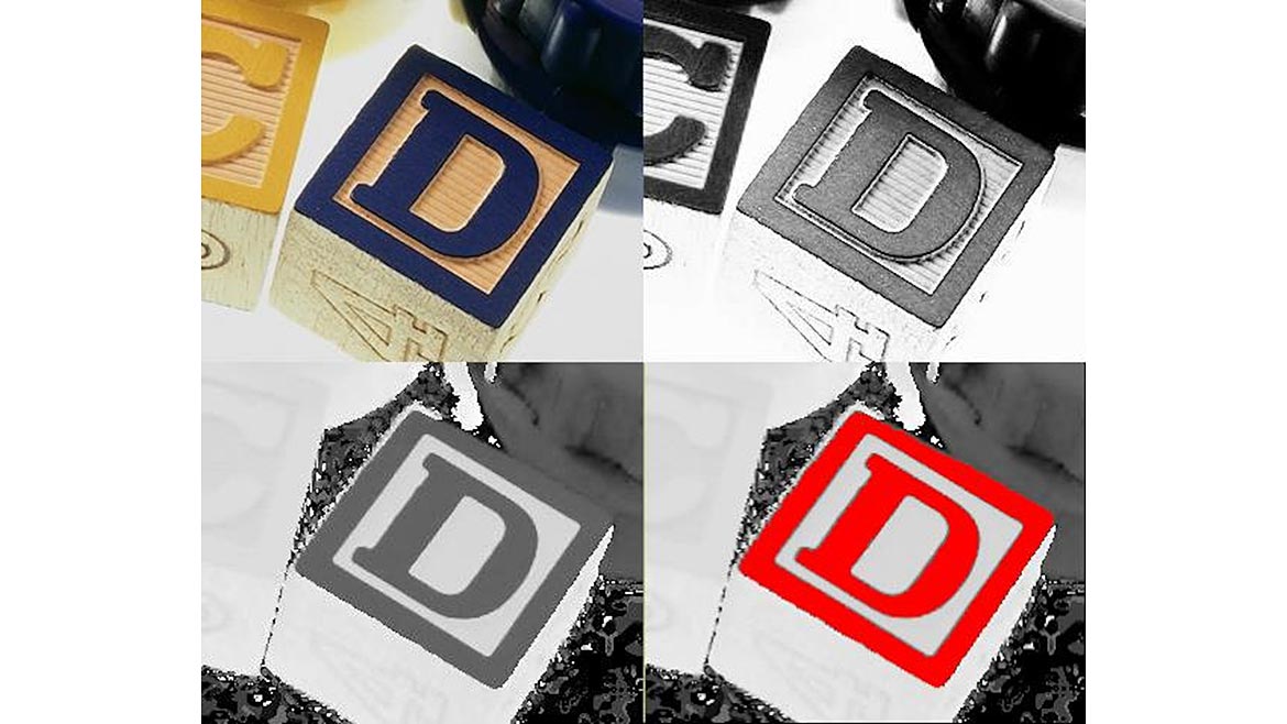
Color analysis in images is most commonly used for differentiation. Examples of this are to confirm that the green part (and not the red part) has been installed on an assembly, or to separate a green part from a red background where there is no differentiation via brightness. Most devices (e.g. screens, computers) record and display color via a combination of red, green and blue (RGB color model) and most processing is done in this color model. But often, a single-color product typically has widely varying RGB values due to inevitable lighting variations but maintains same hue, one of the three parameters that define colors in a different color model (HSI, hue, saturation, intensity) and tools which transform images to that color model enable much better differentiation. For example, in figure 3 it is desired to separate the perimeter and letter in the top face of the blue block for later analysis. While our brains know that the top face is the same color and “see” it accordingly the upper right shows the blue channel which is not consistent. The lower left shows the hue, which is consistent allowing for the separation coded in red in the lower right.  More subtle color inspection requires much more sophistication at the “physics” stage of the solution, sometimes requiring multispectral or hyperspectral imaging.

Gauging (as distinct from blob analysis) consists of taking specific types of measurements at specific places. A simple example is a human drawing two “probes” and measuring between the points where those two probes meet the surface. High accuracy gauging requires much more work at the earlier “physics” stage of the design, but careful work and strong tools during image analysis is also required. Gauging by its nature is done at edges. An edge in an image is granular (being made up of pixels) and a bit fuzzy with gray pixels at the border between the black and white. Gauging tools vary in how they determine where the edge actually is. The simplest methods are threshold based where the edge is taken to be the first pixel encountered by the probe that is darker or lighter than the threshold value. Others use more sophisticated edge models which can even locate the edge with higher resolution than one pixel (sub-pixeling).

If the workpiece moves a large amount between images, those human drawn probes may be in the wrong place on the workpiece or miss it entirely. Location / positioning tools adapt to that. Approaches vary but the common underlying sequence has two stages. During setup a “home” image is chosen, and the software trains itself on where the workpiece is, and the probes are drawn on that home image. Then, at run-time, the software determines how the workpiece has moved (translation, rotation) compared to the home image and moves the probes in the same manner.

One final stage of image processing is producing a pass/fail result, often done by simply counting and evaluating the result. For example, counting the number of oversized surface defects or verifying that one and only one correct part is present in the proper location on an assembly. Often this is the end of the image’s life, but sometimes the image is stored on an automated basis. One example is to document every part. Data such as a serial number or date and time may be coded into the graphics, file name or properties of the image. Another example is conditional storage of only images which failed the inspection. This may provide useful information on defective parts or be used to recreate and solve problems with the operation of the vision solution.

After the image processing is complete, the resultant data is then displayed, transmitted, processed or stored. Hopefully this brief overview of some common functions of the image processing stage has been helpful.