✕

In most production environments, machine operators are responsible for taking samples to monitor the process and empowered to make process adjustments to keep the line running and product flowing. In many cases, they can be reprimanded if they neglect to react to variation in the process. What if the better strategy is to ignore this data and keep chugging along, with no adjustments to the process?

First, let’s discuss our expectations when we sample from a process. Deming outlined his red bead experiment over 40 years ago in his seminal text Out of the Crisis (Massachusetts Institute of Technology, 1982). Imagine a large bucket of beads, mostly white beads with a scattering of red beads well mixed in the bucket. Deming often did this experiment in his seminars, and he would explain that The White Bead Company sells white beads to their customers. He would ask audience members to collect a sample of beads by dipping a paddle with 50 pre-drilled holes, each the right size to capture a bead, into the bucket. An example of possible results is shown in Figure 1, which plots the percentage of red beads collected in each sample (by a given participant). Note first that the number of red beads varied with each participant’s sample. Deming chastised those with a relatively large number of red beads in their sample (“Customers don’t pay for red beads; you’ll be docked pay!”) and congratulated those with a smaller number (“This employee is management material!”). It was all good fun, yet ludicrous, as each participant had zero effect on the number of red beads in their sample. And that was one of Deming’s points: It is ridiculous to grade employees for actions that they have no control over, such as the process design, the equipment, the raw materials, and so on.

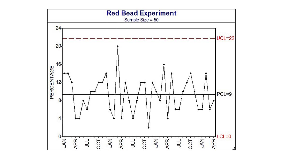
For our purposes here, the samples provide another lesson: Each time we sample from the bucket, we got a different estimate of the percent of red beads, even when the bucket was not changed. Said differently, since the sampling from the bucket is a repeatable process, we should expect to see variation in the sample results, even if that process is unchanged. And when results vary, it does not necessarily mean the process has changed.

If the sample result alone does not tell us the process has changed, how do we know when the process has changed and requires adjustment? Fortunately, there is a tool designed specifically for this purpose by Walter Shewhart, which has been used extensively for over 100 years: the Statistical Process Control (SPC) chart, aka control chart, process control chart or process behavior chart. A properly designed SPC chart will differentiate between those random fluctuations (aka common causes of variation) that are built into a process, and sporadic sources of variation that exceed that expectation. (Shewhart called these assignable causes. Deming referred to them as special causes, acknowledging “the word to use is not important, the concept is…” (Deming, pg.310)).

The concept of detecting a real change in the process implies that time is an important element, as change is something that occurs over time, based on differences between one time frame and the next. Likewise, a process refers to a repeatable set of conditions and activities that occur time after time. A process control chart is always presented with data flowing from the earlier time to the next, so that the variation in the samples from the repeatable process is readily apparent (graphically) and can be conveniently estimated (statistically) over each short time frame.

Shewhart defined the statistical formulas used to calculate the expected variation in the samples, and these are shown in Figure 1, labelled UCL (upper control limit) and LCL (lower control limit). Statistical control limits provide several benefits:

1. Most importantly, statistical control limits provide an operational definition of a special cause: A special cause is present if the sample value is outside the statistical control limits. Think of that old (adapted) Sesame Street lyric: This sample is not like the others; this sample just doesn’t belong. The interpretation of the control chart is that simple.
2. When there are no instances of special cause present, the area between the control limits provides the expected behavior (i.e. our prediction) of the process for the future. In Figure 1, the control limits indicate we should expect the percent of red beads in any sample to be less than 22%. We can use this for planning purposes, such as in budgeting and process capability analysis.
3. Statistical control limits provide a decision rule for action.
    a. When only common causes are present, then no action should be taken based on the value of any current sample. We ignore the sample-to-sample variation within the control limits. If the current process is undesirable, we need to redesign the process to reduce common cause variation.
    b. When a special cause occurs, then we act to determine the conditions currently present that have influenced the process to behave differently. If the new behavior is undesirable, we should seek to remove the condition responsible. If the new behavior is favorable, we should look to standardize on this new condition as a means of process improvement.
4. Control limits provide a statistical basis for the Run Test rules, developed initially by Western Electric as an improvement to the control chart. These Run Test rules provide improved detection of special causes, primarily by looking for patterns in the data within the control limits that are statistically unlikely to occur unless a special cause is present. While these are more cumbersome to use in a paper-based system than the simple comparison to the control limits, when you’re using SPC software to monitor your process, these can be automatically applied for a no-hassle benefit to the chart.

What happens if you’re not using a control chart and you respond to common cause variation as if it were a special cause and adjust or change the process? Deming discussed this using his funnel experiment (Deming, 1982), where he would mark a target on a flat table, then drop a marble from a funnel onto the table from a designated height and note the difference from the drop point to the target. Adjust the process using one of four strategies, and repeatedly use this same strategy for 50 drops. His four adjustment strategies, examples of their use and their results are as follows:

1. Strategy 1: No adjustment to the funnel position. This is the same strategy described for the control chart, where no adjustment is made when the process is influenced by only a common set of conditions. This results in a stable distribution of points, with the minimum possible amount of variation.
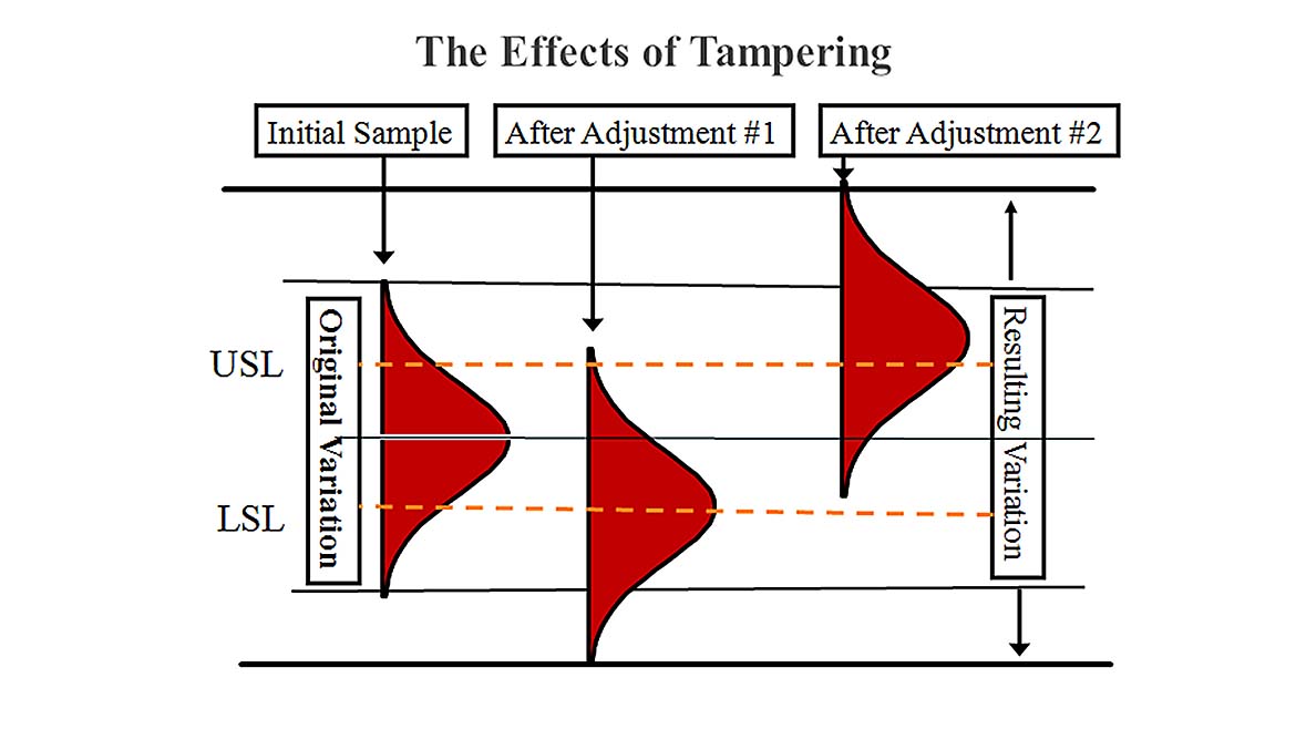
2. Strategy 2: Adjust the funnel position by moving it from the current position toward the target by the amount equal to the difference between the drop point and the target. This is the most common strategy for process adjustment and is illustrated in Figure 2. This occurs when you try to “control” the process using specifications rather than statistical control limits. This tampering with the process results in a stable distribution of points, but with twice the variance experienced via Rule 1. (Mathematically, it can be shown the variance is doubled, which results in the process standard deviation increasing by 40%). In other words: You’ve just increased your defect rate substantially!
3. Strategy 3: Adjust the funnel position by moving it the opposite direction, a distance from the target equal to the difference between the drop point and the target. For example, the most recent data was 20 units above target, so adjust the process by -20 so it will now be on target. This results in ever-increasing (unstable) movement of the process from target, oscillating in one direction then the other.
4. Strategy 4: Adjust the funnel to position it directly over the last drop point. This strategy is more common than you might imagine, with examples cited by Deming including operators who try to reduce variation by making the next piece like the last, or managers who train workers using the recently trained as trainers. This also results in an unstable, ever-increasing movement of the process from target in one direction. This is known statistically as the random walk, which is often described by the metaphor of a drunk trying to walk home, falling at each step, and restarting the next step in a random direction, going further and further off course with each step. Doesn’t end well for the drunk either.

Wheeler recently wrote of the applications of several funnel-type adjustment strategies as they relate to the use of automated PID controllers (Can We Adjust Our way to Quality, Parts 1 & 2, Quality Digest). Many engineers incorrectly surmise that these automated techniques are superior to manual techniques in somehow preventing the entirely predictable increase in process variation due to unnecessary adjustments (noted as Strategy 2, above). Unsurprisingly, his conclusions mirrored Deming’s: The no-adjustment strategy achieves the least variation, whether the process is influenced by common cause variation only or influenced by both common and special causes.

It should be clear that the control chart provides the means to learn about our process.

In fact, it is the fundamental tool of process analysis. No other statistical tool, such as confidence intervals, can be used to estimate process variation, as those tools ignore the element of time, a fundamental aspect of a process. This is the power and exclusive domain of the control chart, which is a necessary precursor for every process improvement activity. Despite your best intentions, you cannot improve a process without first differentiating between common and special causes, as your reaction to each must be different. You cannot effectively implement Lean without the predictability provided by a controlled process. As Deming said: “The distribution of a quality-characteristic that is in statistical control is stable and predictable, day after day, week after week. Output and costs are also predictable. One may now start to think about Kanban or just-in-time delivery.” (Deming, pg. 333).