Top

Calibration laboratories must increasingly utilize clear, defensible decision rules to state conformity, as required by ISO/IEC 17025. Although this is required, many people remain confused about how to implement it in practice. There is little reason not to use these decision rules, as the math behind them is straightforward. This paper presents two robust and user-friendly decision rules: Method 5, whic utilizes Specific Risk, thereby controlling the Probability of False Acceptance (PFA) at each measurement point, and Method 6, also known as the Managed Guard-Band Strategy, which employs Global Risk and was developed by Michael Dobbert.

Choosing a decision rule is a business choice based on risk and consequences. By selecting the right rule, labs can better control the likelihood of making an incorrect decision and meet both their own needs and those of their customers. The paper provides examples, charts, and straightforward advice to illustrate how these decision rules can help laboratories enhance measurements and reduce costs.

1. Introduction

A decision rule, as defined in ISO/IEC 17025:2017, clause 3.7, is a "rule that describes how measurement uncertainty is accounted for when stating conformity with a specified requirement" [1]. While the definition is conceptually straightforward, its practical implementation is often anything but.

Incorrect or ambiguous application of decision rules often leads to costly compliance errors, customer disputes, and inefficient laboratory practices. Thus, establishing clear, robust frameworks for decision-making is critically important for maintaining compliance, minimizing risk, and optimizing laboratory effectiveness.

Many calibration laboratories encounter difficulties implementing decision rules due to inconsistent guidance and the complexity of interpreting standards. Standards typically frame decision rules around managing risk but often assume that end-users clearly understand their measurement uncertainty and how to quantify risk appropriately. This is rarely the case.

Despite foundational documents like JCGM 100:2008, Evaluation of measurement data—Guide to the Expression of Uncertainty in Measurement [2], their depth and complexity make them inaccessible to many practitioners. More accessible references, such as UKAS M3003 [3], have improved understanding; yet challenges remain in achieving a consistent and correct application of measurement uncertainty concepts.

Why is this still a problem? Too often, organizations fail to recognize the operational and financial value of knowing their true measurement capability. The ability to make confident, binary conformity decisions—"Pass," "Fail," or, when justified, "Indeterminate"—depends on integrating measurement uncertainty into the decision-making process.

This paper aims to demystify decision rules and offer a practical pathway forward. Instead of wrestling with an overwhelming array of methodologies (13 plus recognized decision rules, all with their intricacies), laboratories can achieve clarity and compliance by focusing on two well-supported decision rules found in the Handbook for the Application of ANSI Z540.3-2006: Requirements for the Calibration of Measuring and Test Equipment [4].

1. Specific Risk Decision Rule (Method 5): This evaluates the Probability of False Accept (PFA) at the measurement point(s). Specific Risk focuses on the individual measurement result and provides point-by-point guard banding to control risk.
2. The Global Risk Decision Rule (Method 6 or Managed Guard-Band Strategy) employs a standardized risk threshold across all test points, based on the Test Uncertainty Ratio (TUR). Global Risk focuses on a population or the average. (Method 6) that guarantees an upper bound on PFA across the entire range of TUR values—ideal for large-scale calibration programs with varying measurement points.

A clear understanding of the underlying terminology is essential for successfully implementing the decision rules outlined in ISO/IEC 17025:2017. Incorrect or ambiguous application of these rules can lead to costly errors. Precise and robust decision-making frameworks are critical for ensuring compliance, managing risk, and enhancing operational efficiency.

Ultimately, applying a decision rule is not merely a technical exercise—it is a strategic business decision that must harmonize with each party’s unique risk appetite, organizational objectives, and regulatory obligations. It addresses not only the probability of measurement results falling outside specifications but also the broader consequences of those risks to safety, compliance, and operational integrity.

For calibration laboratories, selecting a decision rule reflects their tolerance for Type I (false acceptance) and Type II (false rejection) errors, but it’s equally a reflection of their service philosophy. A lab serving high-reliability sectors, such as aerospace, may adopt guard banding with strict conformity limits, signaling a low-risk appetite and a commitment to conservative metrological decisions. Meanwhile, a lab with a higher tolerance for operational flexibility may choose a decision rule that favors broader acceptance, optimizing turnaround time and cost for clients who are similarly tolerant of low-consequence risks.

On the consumer side, the choice or acceptance of a particular decision rule is an extension of how much residual risk they are willing to absorb in their own processes. A firm producing safety-critical components may demand an "end user guard band" approach, transferring minimal measurement uncertainty into their systems. Another organization may accept a decision rule without guard banding if their internal controls—such as downstream inspections or functional testing—mitigate the impact of potential measurement deviations.

In this sense, the appropriate adoption of decision rules simplifies risk management by embedding clear, aligned tolerances within the calibration process. It creates a shared risk language between the lab and the client, reduces ambiguity in conformity assessment, and strengthens the quality ecosystem.

When thoughtfully chosen, decision rules do more than resolve pass/fail criteria—they promote transparent partnerships, improve overall system reliability, and elevate the laboratory from a transactional provider to a trusted risk management ally.

2. Key Terms and Risk Concepts

• Measurement Uncertainty – A quantified expression of doubt about the measurement result, typically expressed as an expanded uncertainty at a defined confidence level.
• PFA (Probability of False Accept): The likelihood that an out-of-tolerance item is incorrectly accepted.
• PFR (Probability of False Reject): The likelihood that an in-tolerance item is incorrectly rejected.
• EOPR (End of Period Reliability): Historical probability that a measurement remains within tolerance at the end of a calibration cycle.
• ILAC G8:2019/2019 definitions [5]:
• Tolerance Limit (TL or L) (Specification Limit): specified upper or lower bound of permissible values of a property.
• Acceptance Limit (AL): specified upper or lower bound of permissible measured quantity values.
• LAL – Lower Acceptance Limit
• UAL – Upper Acceptance Limit
• Guard band (w): the interval between a tolerance limit and a corresponding acceptance limit, where length w=|TL - AL|.
• Decision Rule: is a rule that describes how measurement uncertainty is accounted for when stating conformity with a specified requirement. (ISO/IEC 17025:2017 3.7 "rule that describes how measurement uncertainty is accounted for when stating conformity with a specified requirement.")
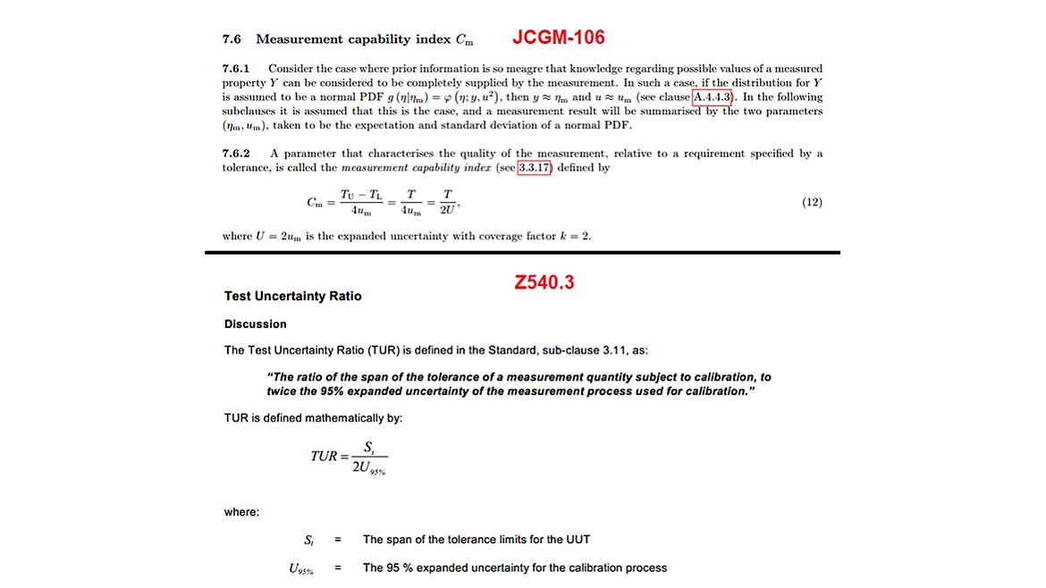
• TUR - the ratio of the tolerance, TL, of a measurement quantity, divided by the 95% expanded measurement uncertainty of the measurement process, where TUR = TL/U.

Note that this definition differs slightly from the one cited in ANSI/NCSLI Z540.3: 2006). The term C_m Measurement Capability Index is virtually identical to this definition of TUR (Appendix A example).

It is crucial to clearly understand these foundational terms, especially Specific Risk (point-based) versus Global Risk (system-based). Misinterpretation can result in incorrect conformity assessments and unnecessary operational costs.

3. Specific vs. Global Risk (ASME Definitions)

ASME B89.7.4.1 defines two distinct approaches for managing measurement decision risk: Specific Risk, focused on individual results, and Global Risk, applied across systems or populations. The table below summarizes these distinctions.

Specific Risk (as defined by American Society of Mechanical Engineers, ASME B89.7.4.1, 2005 [6])

Definition:

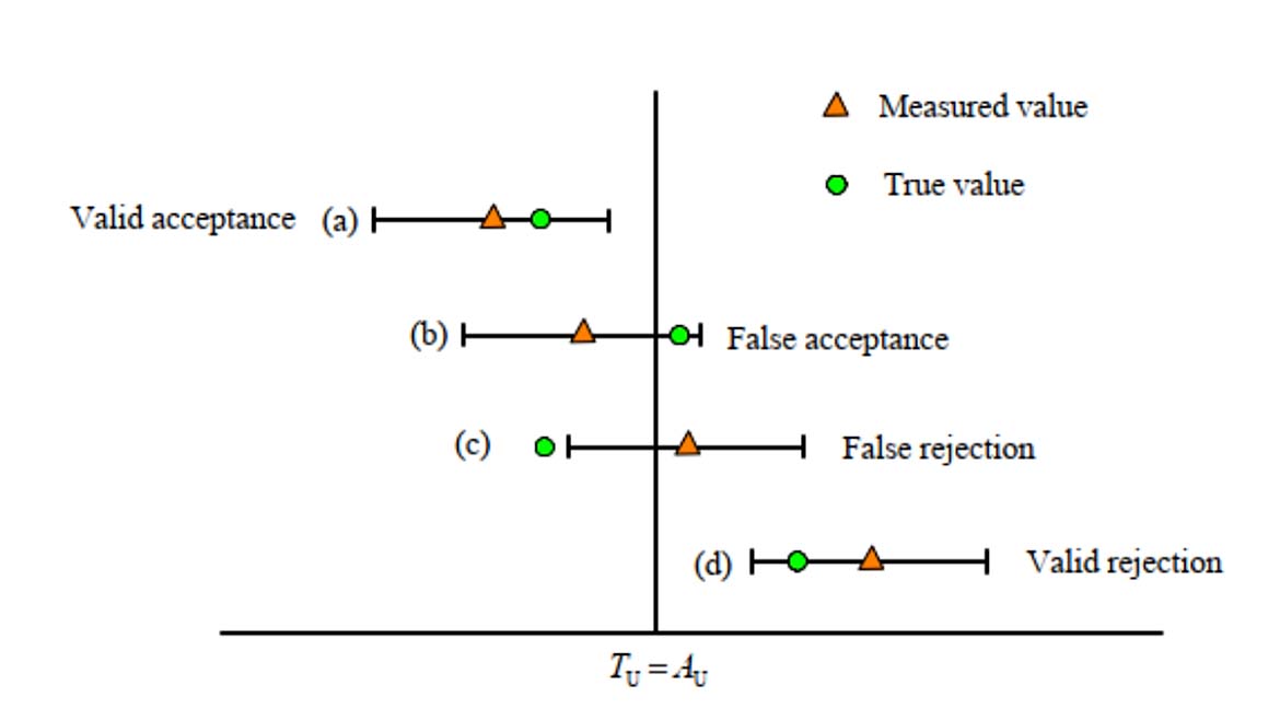
The probability that a specific measurement result lies within the acceptance region while the true value lies outside the tolerance zone.

This is also known as the Probability of False Accept (PFA). It is point-based, calculated at a single test result, and focuses on whether the measured value falsely supports conformity due to measurement uncertainty.

• Specific risk directly depends on the expanded uncertainty and location of the measured value.
• It's evaluated for each individual measurement.
• Often visualized by comparing the overlap between the coverage interval of the measurement result and the tolerance limits.

Used when: tight control is required per test point or when decisions are made at the measurement point.

Global Risk (as defined by ASME B89.7.4.1, 2005 [6])

Definition:

The overall or average probability across a population of measurements that the item will be falsely accepted.

This metric quantifies system-level or population-based risk, measuring the probability of a false acceptance across numerous measurements or calibration cycles.

• Global risk is less sensitive to a single measurement and more concerned with aggregate reliability.
• Often derived using historical reliability metrics like End-of-Period Reliability (EOPR) and Test Uncertainty Ratio (TUR).
• It may use guard band multipliers designed to ensure that the maximum false accept risk across all tests remains below a target, such as 2 %.

Used when: uniform guard bands are applied to many items or test points, or when simplifying risk management across multiple calibrations.

Aspect	Specific Risk	Global Risk	Use Case
Scope	Individual test point	All measurements/system-wide	Point-by-point control
Focus	PFA at a single result	Average/systemic PFA	Aggregate system performance
Calculation Method	From measured value & expanded uncertainty (U)	From TUR/Cm, EOPR, or empirical models	Consistent guard banding
Best For	Critical precision per test point	Uniform guard banding across test sets	High-volume lab operations
Risk Expression	Probability of false acceptance (per point)	Maximum false accept risk (overall)	Ensuring global compliance at <2 % PFA< p>

With this understanding of risk models and terminology, we can now examine how applying these decision rules directly impacts measurement risk, long-term reliability, and the financial dynamics of calibration.

4. Risk, Reliability, and Financial Impact

Assessing calibration costs extends beyond initial estimates. Laboratories often presume consistent test success, yet unforeseen failures and measurement uncertainties can significantly elevate expenses. Failing to address these risks may result in costly recalibrations, adjustments, or operational delays.

For example, a lab calibrating 1,000 units annually could reduce downstream costs by identifying borderline failures early using Method 5 (Specific Risk). In contrast, Method 6 (Global Risk) offers streamlined labor savings across bulk datasets.

Implementing Method 5 (Specific Risk Decision Rule) to assess borderline cases individually can proactively identify instruments that truly fail calibration, thereby avoiding costly downstream errors, reducing potential safety hazards, and safeguarding the laboratory's professional reputation. Early detection of these non-conformances through precise guard banding translates directly into measurable financial savings and customer trust. Conversely, Method 6’s standardized approach streamlines bulk decision-making, significantly reducing labor hours by minimizing the need for detailed inspections on large datasets. This method enhances operational efficiency, allowing the laboratory to allocate resources more strategically and further amplifying overall productivity and cost-effectiveness.

Financial Impact Example:

Using Method 5 (Specific Risk) to assess borderline cases individually might catch instruments that "fail" calibration, potentially saving thousands of dollars downstream and the company's reputation. Conversely, applying Method 6 (Global Risk) could streamline bulk decisions, significantly reducing labor costs by minimizing the time spent on detailed inspections.

Critically, these decision rules ensure compliance with ISO/IEC 17025:2017 clause 7.8.6.2(b), which mandates explicit pass/fail conformity statements without ambiguity - there is no room for "maybe" or "almost." By applying these rules, laboratories deliver precise, definitive results, fully meeting the standard’s requirements [1].

By incorporating financial tools and binary decision rules, laboratories can move beyond compliance checkboxes to a more strategic, risk-based measurement approach that supports quality assurance and cost efficiency.

One of the most effective methods for implementing this strategic, risk-based approach is by choosing a decision rule model that corresponds to an appropriate risk tolerance.

Specific Risk is best suited for applications where a single false acceptance could have serious consequences, such as in aerospace or medical device calibration. This method evaluates the Probability of False Accept (PFA) at each measurement point, enabling precise control and high confidence at the decision boundary. By tailoring guard bands to each result, Method 5 minimizes consumer risk in contexts where accuracy and safety are paramount. However, this increased protection comes at a cost: as PFA is reduced, the Probability of False Rejection (PFR)—also known as producer’s risk—tends to increase.

As a result, laboratories using Specific Risk models may end up rejecting more instruments that are within tolerance, increasing operational costs.

Specific Risk decision rules are most appropriate in scenarios where precision and consumer protection take precedence over cost efficiency.

Global Risk offers a broader, system-level approach ideal for high-volume calibration environments. It applies a consistent guard band strategy across all test points, utilizing metrics such as Test Uncertainty Ratio (TUR) or Measurement Capability Index (C_m), and historical End-of-Period Reliability (EOPR). Instead of assessing individual measurements in isolation, Method 6 (Global Risk) manages aggregate risk, ensuring that the maximum PFA remains below a defined threshold, typically 2%, across the entire calibration program. This approach simplifies decision-making, reduces labor costs, and improves overall operational efficiency without compromising traceable conformity.

Global Risk decision rules are often most appropriate in scenarios where efficiency, consistency, and throughput are prioritized over strict per-point risk controls such as routine calibrations in manufacturing, service labs, or automated systems.

JCGM 106:2012best summarizes this by stating: "Choosing the tolerance limits and acceptance limits are business or policy decisions that depend upon the consequences associated with deviations from intended product quality" [7].

This perspective highlights a critical principle: in the absence of a documented agreement, measurement uncertainty is generally assumed to count against the party asserting conformity, whether that be the laboratory, manufacturer, or regulator.

Taken together, the Specific and Global Risk models offer laboratories a flexible framework for aligning conformity assessments with technical risk tolerance, operational needs, and customer expectations. However, regardless of the decision rule chosen, all accredited laboratories must ensure that their conformity assessment statements adhere to the requirements outlined in ISO/IEC 17025. This includes applying decision rules in a way that produces clear, unambiguous, and defensible results. The following section examines how ISO/IEC 17025 mandates the use of binary decision language and explains why this is important for both regulatory compliance and customer trust.

5. Binary Decision Rules and the Role of ISO/IEC 17025

ISO/IEC 17025:2017, clause 7.8.6.2(b), states:

"The laboratory shall report on the statement of conformity, such that the statement identifies:

1. ) to which results the statement of conformity applies;
2. ) which specifications, standards, or parts thereof are met or not met;
3. ) the decision rule applied (unless it is inherent in the requested specification or standard)[1].

Though this language may not have been written explicitly to do so, it effectively precludes the use of vague or non-binary conformity statements. Terms like "Pass (Indeterminate)" or "Fail (Conditional)" introduce ambiguity into conformity decisions and fall outside the scope of ISO/IEC 17025–compliant reporting. The standard is clear: conformity must be stated in binary terms—Pass or Fail, Met or Not Met. If a laboratory chooses to use non-binary terms, it cannot, by definition, label the result a valid "statement of conformity."

JCGM 106:2012 reinforces this position by emphasizing that conformity decisions are probabilistic and must be made using defined acceptance intervals. It warns that, "because of uncertainty in measurement, there is always the risk of incorrectly deciding whether or not an item conforms" [7, Clause 6.3.2.3]. Introducing non-binary language blurs that decision boundary and undermines the integrity of the decision rule applied. Worse, as JCGM 106 outlines in its treatment of acceptance and rejection zones, failure to clearly define the outcome increases the risk of false acceptances or rejections—precisely the risks conformity assessment systems aim to control.

ISO/IEC 17025:2017, Clause 7.1.3 further reinforces this by requiring that:

"When the customer requests a statement of conformity to a specification or standard for the test or calibration (e.g., pass/fail, in-tolerance/out-of-tolerance), the specification or standard and the decision rule shall be clearly defined.[1]"

This requirement reinforces the need for well-defined decision rules, particularly those like Method 5 (Specific Risk) and Method 6 (Global Risk, aka Dobbert’s Rule), that produce unambiguous outcomes. When measurement risk is managed correctly and uncertainty is transparently accounted for, laboratories are better equipped to meet this binary standard of conformity, reducing liability and improving trust in the reported results.

Comparing Method 5 (a specific risk method) to a global risk methodology (single vs. joint probability) highlights a flaw: it’s incorrect to label a test point as a "pass" globally while calling it "indeterminate" under Method 5. Though ISO/IEC 17025 doesn’t explicitly allow non-binary terms, an "Indeterminate Pass" might be justified in rare cases—like a pass under Method 6 (Global Risk) but a failure under Method 5—to show decision rule divergence transparently. This requires prior definition and agreement. Post hoc rule selection by customers (e.g., "give me whatever passes") compromises impartiality and must be avoided. A single, pre-set decision rule ensures compliance and consistency.

6. Overview of Method 5 (Specific Risk) and Method 6 (Global Risk)

Specific Risk refers to the probability that a particular measurement result falls within the acceptance zone while the true value is out of tolerance. This is commonly called the Probability of False Accept (PFA).

6.1 Method 5 (Specific Risk) Example: Two-Sided Guard Bands

There are numerous methods for calculating acceptance limits. The method presented below applies to any level of risk. If the stakeholder says they want a 10% risk, it works; if they want a 1% risk, it works. Therefore, this is the de facto method for calculating specific risk.

ASME B89.7.4.1 2005 [6] provides an explicit method of setting the width of the acceptance zone for a specified probability of conformance.

The Guard band is a multiple of the expanded uncertainty of the measurement process, g=hU, where the Guard bands are the same size, gL = gU = g. The guard band multiplier (h) is given by:

h=1/2 ϕ^(-1) (P_C )

Formula to Calculate Specific Risk.

Where:

Φ-1  ( ) is the inverse standard normal distribution function—the Excel function to calculate  Φ-1 NORM.S.INV.

h is the guard band multiplier

U  is the Expanded Uncertainty

Pc is the probability of conformance

GU is TU – hU

TU is the Upper Tolerance Limit

The Guard Band is chosen so that a desired portion of the probability of conformance area under the curve lies inside the tolerance zone. ASME B89.7.4.1-2005 "Measurement Uncertainty and Conformance Testing: Risk Analysis," Section 8 [6].

Example Specific Risk Acceptance Zone Calculations – Two-Sided

In this example from Decision Rule Guidance 1^st Edition, V1.3, 2024 [8], we are trying to calculate the acceptance zone using a guard band to limit our risk to a 2.5 % limit between -1 (Lower Tolerance Limit) and + 1 (Upper Tolerance Limit) units with a standard measurement uncertainty of 0.125 units.

Our Standard Measurement Uncertainty (k = 1) is 0.125 units.

This Standard Measurement Uncertainty is applied as Expanded Measurement Uncertainty at a Coverage Factor of 2 to express at a 95.45 % Confidence Interval, assuming infinite degrees of freedom.

The customer has instructed us to reject anything with a risk of more than 2.5 % per side.

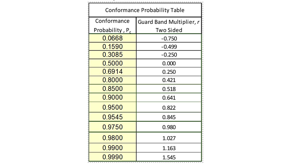
Thus, we are calculating our Conformance Probability for 97.50% (100% - 2.5%) confidence for a symmetrical tolerance. We calculate the guard band Multiplier using the Excel formula NORM.S.INV(0.975)/2, which results in 0.980.

We then use this value of 0.980 as our GB Multiplier as follows.

For the guard band upper limit, we have 1 – (GB Multiplier * Coverage Factor * Standard Measurement Uncertainty)

1 – (0.980 * (2 * 0.125)) = 0.7550

For the guard band lower limit, we have -1 + (GB Multiplier * Coverage Factor *Standard Measurement Uncertainty)

-1 + (0.980 * (2 * 0.125)) = -0.7550

Our Acceptance Zone is to pass any measured value between -0.7550 and + 0.7550 [8].

The formula can be simplified to:

Acceptance Limit = Tolerance Limit ± Guard band multiplier * Expanded Measurement Uncertainty.

ILAC-G8:09/2019 states, "Often the Guard band is based on a multiplier r of the expanded measurement uncertainty U, where w = rU. For a binary decision rule, a measured value below the acceptance limit AL = TL–w is accepted. [5]"

6.2 Method 5 (Specific Risk) Example: One-Sided Guard band

We are trying to calculate the acceptance zone using a guard band to limit our risk to a 5% limit between a lower tolerance and an upper tolerance. In this example, we use either -1 (Lower Tolerance Limit) or + 1 (Upper Tolerance Limit) units with a standard measurement uncertainty of 0.125 units.

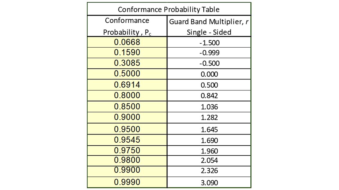
We are calculating our Conformance probability for 97.50% Confidence using a single-sided tolerance. We calculate the guard band Multiplier using the Excel formula of NORM.S.INV(0.975).

Our Standard Measurement Uncertainty (k=1) is 0.125 units.

This Standard Measurement Uncertainty is applied as Expanded Measurement Uncertainty at a Coverage Factor of likely 2 to express an approximate 95% Confidence Interval, assuming infinite degrees of freedom.

Thus, we are calculating our Conformance Probability at 97.50% (100% - 2.5%) confidence. We calculate the guard band Multiplier using the Excel formula of NORM.S.INV(0.975), which results in 1.960.

We then use the number 1.960 as our GB Multiplier as follows.

If the single-sided tolerance is an upper tolerance:

For the Guard band upper limit, we have 1 – (GB Multiplier * Coverage Factor * Standard Measurement Uncertainty)

1 – (1.960 * (2 * 0.125)) = 0.51

If the single-sided tolerance is lower:

For the Guard band lower limit, we have -1 + (GB Multiplier * Coverage Factor *Standard Measurement Uncertainty)

-1 + (1.960 * (2 * 0.125)) = -0.51

The formula can be simplified to:

Acceptance Limit = Tolerance Limit ± Guard band multiplier * Expanded Measurement Uncertainty [8].

The Managed Risk Guard band leverages the measurement capability index (C_m) to cap consumer risk across all product and process uncertainty levels.

A notable behavior occurs when C_m drops below 1:1 (i.e., when measurement uncertainty equals or exceeds the tolerance). In this region, the PFA curve declines sharply. At first glance, this may appear counterintuitive. Why would the risk of false acceptance decrease when the measurement quality is poor (Figure 5)?

The reason this happens is related to how the decision rule operates. When TUR/C_m is low, the guard band gets wide, and the range where something can "pass" becomes very small. That means it’s much harder for anything to pass the test. Most items get marked as "fail," not because they’re bad, but because there’s too much uncertainty to be sure they’re good. So, the chance of wrongly passing something (false acceptance) goes down, not because the test is more accurate, but because nearly everything gets rejected just to be safe. This protects the customer but can unfairly hurt the manufacturer.

The above assumes a worst-case TUR (Figure 6). When both True EOPR and TUR are low, most measurements lie outside of the tolerance, and the risk of falsely accepting an item is low. The false acceptance risk is low when EOPR is near 100%. It is less than 2% when the true EOPR is ≥ 95% (True EOPR is the actual value that is not assumed or modeled).

Therefore, applying just enough of a guard band to lower the maximum risk below a desired level is possible for a given measurement capability index C_m.

Thus, Dobbert calculated a multiplier that adjusts the guard band for a specified measurement capability index (C_m) to meet the 2% consumer risk requirement of Z540.3.

This method ensures that consumer risk is minimized while maintaining control over producer risk.

Applying a guard band to manage maximum false-accept risk results in a guard band that is always less than the 95% expanded uncertainty. Accordingly, the acceptance limits can be expressed as follows,

A = T −U95 % × M

Where:

A = acceptance limit

T = tolerance limit

U95 % = calibration process 95% expanded uncertainty

M = multiplier: the fraction of the 95% expanded uncertainty for which the acceptance limits provide the desired false-accept risk.

M_{2 %} = 1.04 – e^{((0.38 ln(Cm) – 0.54)}

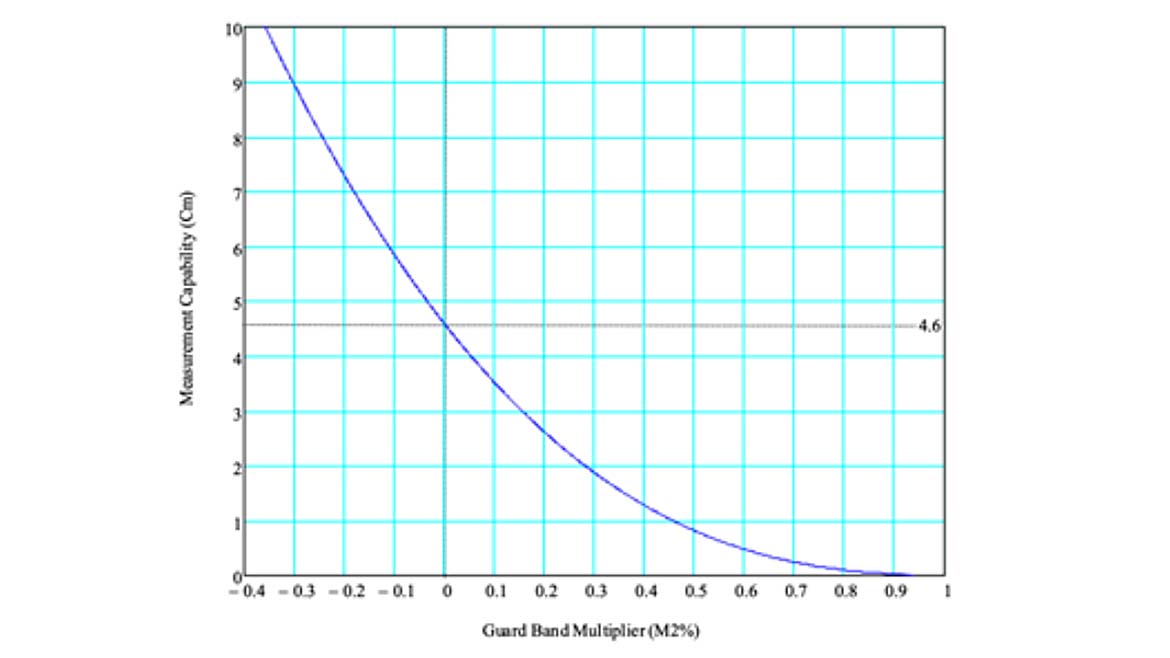
This graph (Figure 7) plots the guard band multiplier (M2 %) on the x-axis against measurement capability index (Cm) on the y-axis. It is used to determine the size of a guard band needed to control consumer risk (specifically, to maintain a maximum false accept risk of 2 %) in Method 6 (Global Risk) decision rules, often referred to as Dobbert’s Rule.

A = T −U95 % × M

C_m = Measurement Capability Index (TUR)

M = 1.04-EXP(0.38 x ln(C_m)-0.54)

T = Required Tolerance

Calculation of TUR/C_m

Note: Method 6 (Managed Guard Bands) is intended for symmetrical two-sided tolerances only; it is not applicable to single-sided or asymmetrical tolerances.

Method 6 Example: Global Guard Band Application

M_(2%)=1.04-exp(0.38×ln⁡(TUR)-0.54)

+Acceptance=Upper Test Limit-Uc95%×M_(2%)

-Acceptance=Lower Test Limit+Uc95%×M_(2%)

Test Limit (TL)= ±1

Expanded Measurement Uncertainty (Uc95 %) = ±0.5

TUR = 1/ 0.5 = 2.0

M_(2%)=0.281 645 308 

+ Acceptance Limit = Upper TL - Uc95%×M_(2%)= 0.859 177 346

-Acceptance Limit = Lower TL +  Uc95%×M_(2%)= -0.859 177 346

The M 2% expression was empirically fit to achieve a worst-case PFA of 2%. This method is straightforward to apply, providing offers consistent risk reduction across various TURs.

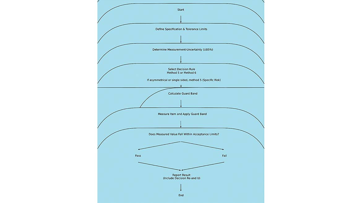
7. Flowchart

8. Conclusion

Many labs struggle with making clear "pass" or "fail" decisions because the rules about how to handle measurement uncertainty are often confusing. Yet it doesn’t have to be that way.

Practically, laboratories adopting these decision rules have demonstrated reductions in compliance incidents, decreased overall calibration costs, and improved operational efficiency.

This paper details two decision rules: Method 5 (Specific Risk) and Method 6 (Global Risk). Method 5 (Specific Risk) scrutinizes each measurement to reduce the likelihood of accepting non-compliant items. Method 6 (Global Risk) employs a comprehensive strategy, maintaining low risk across numerous tests.

These rules facilitate adherence to standards such as ISO/IEC 17025 and streamline conformity assessments, eliminating ambiguity with definitive pass/fail results, not "maybe" or "perhaps."

Method 5 and Method 6 offer defensible, standards-aligned approaches to conformity assessment. Their adoption improves clarity, reduces risk, and supports both operational and financial performance. When laboratories or industries implement these methods, they often realize significant cost savings. Choosing to adopt Method 5 (Specific Risk) or Method 6 (Global Risk) is ultimately a business decision based on evaluating risk and its consequences. Both methods have proven effective in technical and operational contexts.

Companies without structured decision rules should adopt Method 5 (Specific Risk), Method 6 (Global Risk), or both. Integrating these rules with emerging calibration technologies and assessing their performance in specific industries will validate their effectiveness, drive continuous improvement, and deliver measurable operational and financial benefits.

References

[1] ISO/IEC 17025:2017, General Requirements for the Competence of Testing and Calibration Laboratories. ISO, Geneva, Switzerland, 2017.
[2] JCGM 100:2008, Evaluation of Measurement Data—Guide to the Expression of Uncertainty in Measurement (GUM). BIPM, Sèvres, France, 2008. [Online]. [3] UKAS M3003, The Expression of Uncertainty and Confidence in Measurement, 4th ed., United Kingdom Accreditation Service, Feltham, UK, 2019.
[4] NCSLI, Handbook for the Application of ANSI Z540.3- 2006: Requirements for the Calibration of Measuring and Test Equipment, NCSL International, Boulder, CO, USA, 2009.
[5] ILAC G8:09/2019, Guidelines on Decision Rules and Statements of Conformity, International Laboratory Accreditation Cooperation, Silverwater, Australia, 2019.
[6] ASME B89.7.4.1-2005, Measurement Uncertainty and Conformance Testing: Risk Analysis, American Society of Mechanical Engineers, New York, NY, USA, 2005.
[7] JCGM, Evaluation of measurement data — The role of measurement uncertainty in conformity assessment, JCGM 106:2012, Joint Committee for Guides in Metrology, 2012.
[8] G. Cenker, H. Zumbrun, and D. Shah, Decision Rule Guidance v1.3, Morehouse Instrument Company, York, PA, USA, 2022.
[9] P. Reese, "False Accept Risk and Binary Decision Making," NCSLI Measure, vol. 17, no. 3, 2022.
Appendix A
Additional Information supporting TUR is mathematically identical to Cm.
Looking for a reprint of this article?
From high-res PDFs to custom plaques, order your copy today!